Freie Universität Berlin

A simple example.

Calling Python from within R via the R-package rPython is fairly easy. However, very little documentation exists on this package, and some of the commands may appear quirky at first. Also, don’t confuse rPython with RPython (see capitals)! The paucity of written documentation on this package seems to scare away many biologists, who – if they are like me – prefer to work with well-documented code. But fear not!

Usage of rPython is straightforward with a bit of exercise. The following tutorial is intended to give a quick and simple example on how to work with rPython.

I use the command python.exec() to execute basically any Python operation within R.

I use the command python.get() to assign a new variable in R with a value from Python.

Note, however, that python.get() is very inflexible in what it can retrieve from Python.

Instead, I use:

A helper script in R

I recently needed to concatenate multiple .csv-files, which displayed the same row names. The concatenated matrix would thus consist of columns from different files. To that end, I wrote the following R script.

First, let us specify the input directory.

Second, let us list all .csv-files in the input directory and load the first file.

Third, let us loop through all other .csv-files and attach them to the growing dataframe.

Fourth, let us order the rows of the final matrix according to the very first .csv-file, and then save the matrix as output.

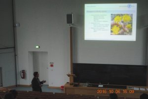
Today, different groups of the Dahlem Center of Plant Sciences met for their annual symposium, the DCPS Day 2016. It was a great symposium, and I enjoyed giving my presentation to this great set of research groups.

Presentation at DCPS Day 2016

Yesterday, a few colleagues and I went on an excursion to the Döberitzer Heide, an anthropogenic heath in the state of Brandenburg.

Flower of Verbascum densiflorum (Scrophulariaceae)

Tachina fera on Knautia arvensis (Dipsacaceae)

 
.

Facilitating their transition to college

As part of the Summer University 2016, a unique course by the Freie Universität Berlin that allows high-school students to attend college-type lectures, I organized a lecture session on plant evolution today. Lots of interested students and good questions afterwards!

Sommeruni 2016 – 23 Aug 2016

The issue with hardcoding data formats

Various phylogenetic analyses in R work on the ultrametric trees generated by the popular software BEAST. In order to load such trees (including their node metadata) into R, the R packages phyloch and, more recently, ips provide useful tree and data parsers. Specifically, the parsing of the input trees is conducted with function read.beast(), which reads NEXUS files as saved by the BEAST components (e.g., TreeAnnotator) or related software.

Recently, I realized that node metadata can only be loaded with the above-mentioned R function if the tree name in the NEXUS tree definition line starts with “TREE1″. This specification is hard-coded in the dependent function extractBEASTstats(), which parses the node metadata from each tree.

See lines 2 and 3 of function extractBEASTstats():

I am not certain if there is a convention that all tree names in BEAST-generated NEXUS files must start with the string “TREE1″. However, future data parsers for BEAST should probably avoid this specific condition, as successful parsing should not depend on a specific tree name.

A helpful note

Saving text elements via the default svg-drivers of R (e.g., grDevices::svg, Cairo::CairoSVG) often results in the text being saved as paths instead of genuine text elements. Downstream svg-editors (such as Inkscape) may thus only allow you to move single letters but not edit them as text elements (which slashes the point of being a text element).

Fortunately, the R package svglite contains an svg-driver that saves text elements as such.

Compound but not complex

The Biopython manual informs the alert reader that ‘join’ locations of EMBL/GenBank files can be handled by CompoundLocation objects. This class of objects is a special object class in Biopython and very straight forward to operate.

Assume, for example, the following DNA sequence:

This example sequence contains three exons (each 3-bp long), which are flanked by 2-bp long spacers that have the sequence “AA”. Taken together (i.e., ‘joined’), they translate to the following protein consisting of two aminoacids: “M I *” (where the asterisk indicates a stop codon). How can I extract the exons from the above sequence?

First, you set up three FeatureLocation objects:

Second, you convert the FeatureLocation objects to a CompoundLocation object:

Third, you extract the exons from the sequence via the CompoundLocation object:

Finally, you translate the extracted DNA sequence:

QED.

The truth that any writer (scientific or otherwise) comes to understand:

“That’s the magic of revisions – every cut is necessary, and every cut hurts, but something new always grows.”

(attributed to author Kelly Barnhill)

Better parallel than serial

In one of my past projects, I implemented the usage of multiple CPUs for time-intensive phylogenetic computations. I hereby used the R library Rmpi for the coordination of parallel processes. Rmpi is an R wrapper for the MPI communications protocol. The speed gains that my code execution was experiencing through this process parallelization was considerable, and it may, hence, be of interest to a wider audience. I therefore present here a small example of using Rmpi in phylogenetic investigations.

First, let us set up a set of calculations that warrant process parallelization. In a maximum parsimony tree search, for example, multiple starting trees may wished to be evaluated. A parsimony ratchet can be executed in parallel on these starting trees, as the runs are independent of each another.

Second, let us execute the parsimony ratchet serially (where an MP analysis is executed with the first starting tree, then the second, then the third, etc.). As we can see, MP inference performed serially on my data set takes roughly 10 min.

Third, let us execute the parsimony ratchet in parallel, using the maximum number of CPUs available on my system (nproc = 8). As we can see, the MP inference performed in parallel on my data set takes roughly 4 min.

Utilizing all 8 CPUs on my computer (one for the master process, the rest for the slave processes) is not necessarily the most efficient parallelization. Spawning each slave process requires a certain amount of CPU resources, and these resources may be larger than the benefit of the added calculation speed (i.e. law of diminishing returns).