Freie Universität Berlin

A post without spello in the title

Today, I attempted to blast entire chloroplast genomes against NCBI’s nucleotide database via the BLASTn command-line tool. Since typical plastomes are between 150,000 and 160,000 bp in length, BLASTn searches that are conducted remotely take approximately 20 min. on average.

time blastn -db nt -query myinputseq.fasta -remote -out results.txt

real 21m25.189s
user 0m0.070s
sys 0m0.010s

Can we speed up such searches by splitting the input query sequence into equally-sized, smaller pieces and blasting each piece separately?

# Splitting input query sequence into ten equally-sized, smaller pieces

INF=myinputseq.fasta
split -d -b $(bc <<< $(tail -n1 $INF | wc -c)/10) $INF prt

# Blasting each region against NCBI’s nucleotide database

for i in $(ls prt*); do
echo $i >> results.txt;
time blastn -db nt -query $i -remote -outfmt '7 length pident sscinames' -max_target_seqs 10 -out $i.result >> time.txt;
rm $i;
done


real 0m15.161s
user 0m0.060s
sys 0m0.010s

real 0m28.901s
user 0m0.060s
sys 0m0.013s

real 0m27.328s
user 0m0.057s
sys 0m0.013s

real 0m14.909s
user 0m0.067s
sys 0m0.010s

real 0m13.689s
user 0m0.043s
sys 0m0.023s
etc.

Yes, we can! (However, I bet that the above scenario was a lucky incidence, and that the time improvement caused by reducing the query sequence size is not always that pronounced).

Following the German motto “Ordnung ist das halbe Leben!”

Have you ever been frustrated by having to differentiate between dozens of similar graphs or figures, and the only memorable difference between them were their unique file names?

In a recent simulation study, I had exactly that feeling, so I came up with some code to automatically label figures with their file names. Here is how it works:

For example, please assume three similar graphs with the file names testResults_A.png, testResults_B.png, and testResults_C.png, respectively.

testResults_A

testResults_B

testResults_C

Let us annotate each figure automatically with its file name (but excluding the file type ending) using ImageMagick.

On the top of each figure, an orange bar with the respective file name has now been added.

annotated testResults_A

annotated testResults_B

annotated testResults_C

UPDATE: I found it necessary to manually set the font size in several cases. It is hereby important to set option pointsize as the first option in the list.

A quick R example

Today, I needed to convert a series of state matrices into presence-absence matrices. In order to automate this conversion, I wrote the following R code. (The initiated will recognize the output as a species-range matrix.)

1.a. Generate example input

m = matrix(data=c("A","B","C"), nrow=3, ncol=1)
rownames(m) = c("t1", "t2", "t3")
m
[,1]
t1 “A”
t2 “B”
t3 “C”

1.b. Alternatively, one could load a table from file

t = as.matrix(read.csv("~/test.csv", header=FALSE))
m = as.matrix(t[,2])
rownames(m) = t[,1]


2. Generate the presence-absence matrix

l = length(unique(m[,1]))
m = cbind(m, matrix(rep(0,l), nrow=nrow(m), ncol=l))
colnames(m)=c(NA,c(unique(m[,1])))
for (i in c(unique(m[,1]))) {m[which(m[,1] %in% i), i]=1}
m = m[,-1]
m
A B C
t1 “1” “0” “0”
t2 “0” “1” “0”
t3 “0” “0” “1”

EDIT: If any of the entries in the state matrix were to contain a combination of states (e.g., “A and B”), the following code should be used at step #2:

tmp = unique(m[,1])
new = tmp[-which(tmp==tmp[grepl(" and ", tmp)])]
addon = unlist(strsplit(tmp[grepl(" and ", tmp)], ' and '))
ul = unique(c(new,addon))
l = length(ul)
m = cbind(m, matrix(rep(0,l), nrow=nrow(m), ncol=l))
colnames(m)=c(NA,ul)
for (i in ul) {m[which(grepl(i, m[,1])), i]=1}
m = m[,-1]


Working at the intersection

I have always wondered why an Illumina machine occasionally generates “unpaired” paired-end reads (i.e., when you receive an R1 but no corresponding R2, or vice versa). While I am waiting for a satisfactory answer, I would like to remove any unpaired reads from my data set in the meantime.

Superficially, this aim may appear to be achieved through joining paired-end Illumina reads, which can be done through several software tools (e.g., FastqJoin). In reality, however, all I wish to do is to filter out unpaired paired-end reads. Such a task is best completed by some shell scripting.

First, I define my infiles.

INF1=infile_R1.fastq
INF2=infile_R2.fastq


Second, I check if any unpaired paired reads are present.

c1=$(wc -l $INF1 | awk '{print $1}')
c2=$(wc -l $INF2 | awk '{print $1}')
if (($c1 == $c2)); then echo "TRUE"; else echo "FALSE"; fi


Third, I extract the sequence names (but not the actual sequences, nor the quality scores).

cat $INF1 | grep '^@' | grep -v ',' > $INF1.headers
cat $INF2 | grep '^@' | grep -v ',' > $INF2.headers


Fourth, I remove the unique pair-identifiers from the end of all sequence names. (This may vary depending on your data.)

sed -i 's/\_1\:N\:0\:3//g' *.headers
sed -i 's/\_2\:N\:0\:3//g' *.headers


Fifth, I list all intersecting elements.

comm -12 $INF1.headers $INF2.headers > intersect.headers


Sixth, I extract those reads from the input files, whose sequence names appear in the intersection. (Unfortunately, this step is slow. If anyone can come up with faster code, please write me.)

for i in $(cat intersect.headers); do cat $INF1 | grep -A3 ^$i >> $INF1.intersect; done &
for i in $(cat intersect.headers); do cat $INF2 | grep -A3 ^$i >> $INF2.intersect; done &

Seventh, I perform some file hygiene.

rm *.headers

You then continue to work with the filtered files $INF1.intersect and $INF2.intersect, respectively.

EDIT: Upon bouncing some ideas off of Stackoverflow, I found a much faster code to conduct step 6 of the above pipeline (i.e., extracting those reads from the input files, whose sequence names appear in the intersection). Hence, the following code should be used instead:


grep -A3 -Ff intersect.headers $INF1 >> $INF1.intersect &
grep -A3 -Ff intersect.headers $INF2 >> $INF2.intersect &


 “On the Birds and the Bees” for botanists

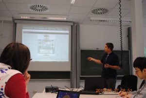
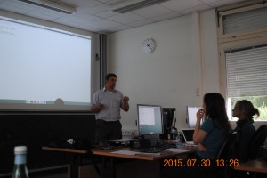
Currently, I am teaching a class on the biodiversity and evolution of flowering plants, particularly from a phylogenetic perspective. I love academic teaching, and I hope my students enjoy the course as much as I do.

Teaching – July 2015

Teaching – July 2015

Priming for success

It has been several years since I last developed a pair of customized oligonucleotide primers for DNA sequencing. At that time I tended to operate software via GUIs, not knowing that an entire toolkit of commandline tools exists, which can get the job done faster and more efficiently. Today I have an opportunity to explore this toolkit.

Assume that you have (a) a tab-delimited database of oligonucleotide primers (e.g., primer_database.tsv), and (b) a fasta-formatted DNA alignment of a target organism (e.g., target_alignment.fas). Your primer database contains hundreds of primers, each occupying one line and followed (on the same line) by information regarding the target gene (e.g., matK) or the strand orientation (e.g., R for reverse). How can you identify those primers within your database that will likely bind to one or more of the target organism?

First, you extract your primers of interest via grep and awk.

cat primer_database.tsv | grep matK | grep $'\tF\t'
| awk -F '\t' '{print $2, $3}' > matK_forw.tsv


Second, you loop through your primers of interest and match them to the target alignment via fqgrep, allowing a specified number of mismatches.

for i in $(cat matK_forw.tsv | awk '{print $2}'); do fqgrep -m 1
-p $i -r target_alignment.fas >> forward_oneMismatch.txt; done


Third, you reduce the resulting list of matches so that extraneous information is filtered out and all matches are combined into a single text file (e.g., combined.txt).


for i in $(ls *Mismatch.txt); do echo $i >> combined.txt; cat $i
| awk -F '\t' '{print $1, $3, $7, $8, $9}' >> combined.txt;
echo "\n" >> combined.txt; done


You now have a list of primers that match the target sequences and can evaluate other factors relevant to the design of oligonucleotide primers, such as amplicon length, melting and annealing temperatures, and hairpin and dimer formation.

P.S. Special thanks goes to my colleague Nadja K. for reminding me of relevant issues involved in primer design.