
Image metadata can be both scary and useful
Assume that you are a field botanist on an expedition and that you take photographs of every collection site that you visit. The metadata that is routinely stored as part of your photograph can be used to visualize your collection sites on a map. For example, the following photograph that I took while collecting plants on a bike trip has the following GPS metadata:
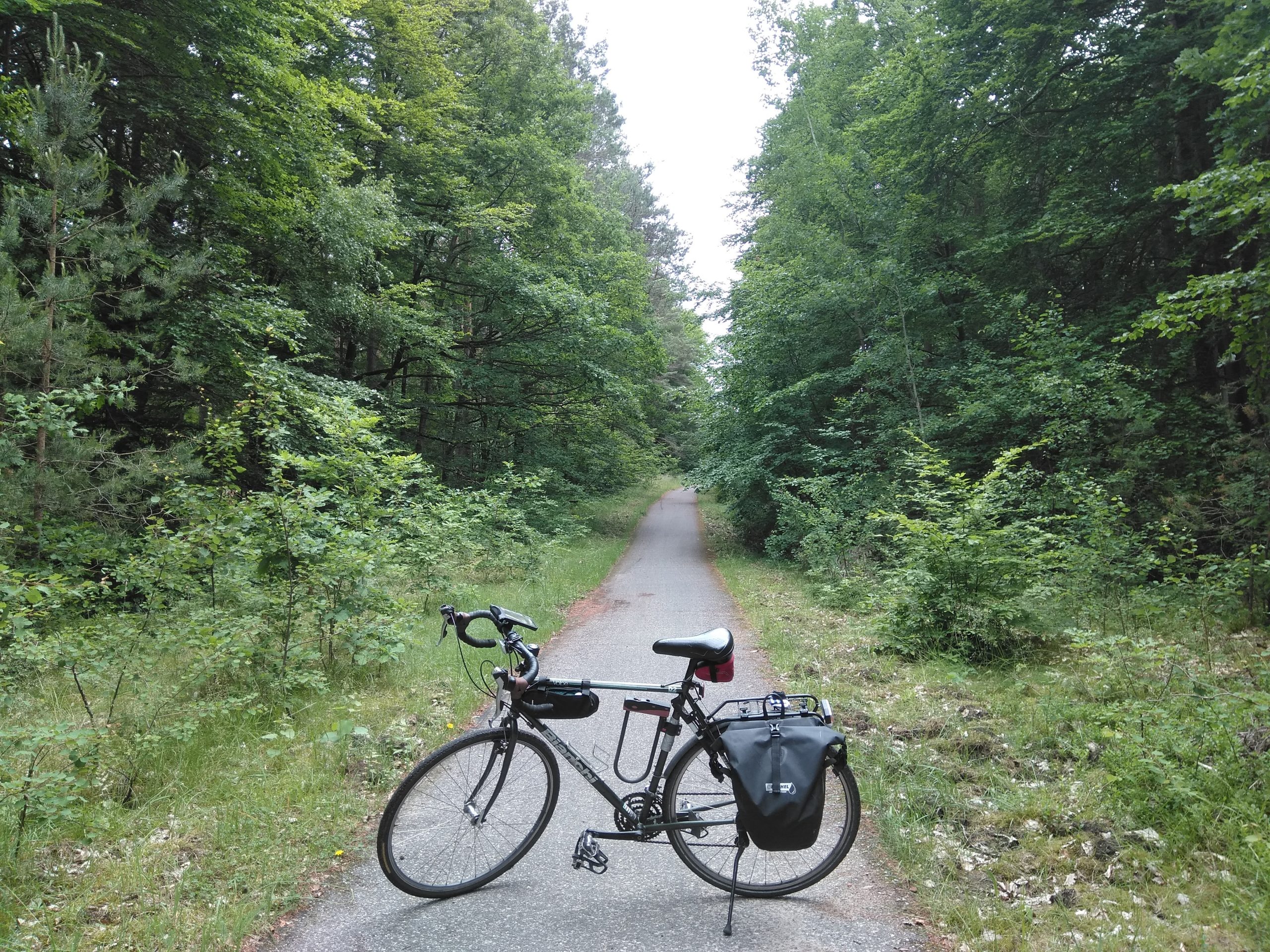
Field trip by bike near Neuruppin
GPS Latitude Ref           : North
GPS Longitude Ref          : East
GPS Altitude               : 123 m Above Sea Level
GPS Date/Time              : 2019:06:21 14:57:30Z
GPS Position               : 53 deg 8' 56.52" N, 13 deg 14' 18.04" E
A visualization via picture metadata is quite easy to achieve with R.
First, you use the R package exiftoolr to parse and extract the GPS metadata that may be stored as part of your field trip photographs. Notice that I use the function exif_read() to parse the metadata from all images in the image folder and that I remove all cases where no metadata was extracted from the images via function na.omit().
library(exiftoolr)
inData = exif_read(path="/path_to_image_folder/",
   recursive=TRUE,
   tags=c("FileName", "GPSDateTime","GPSLatitude", "GPSLongitude"))
inData = as.data.frame(inData)
inData$SourceFile <- NULL
locs = na.omit(inData[,c("GPSLatitude","GPSLongitude")])
Second, you use the R package ggmap to download a suitable map and to plot the latitude and longitude information that you extracted from the image metadata onto that map.
library(ggmap)
lowerleftlon = min(locs[,2])-6*sd(locs[,2])
lowerleftlat = min(locs[,1])-2*sd(locs[,1])
upperrightlon = max(locs[,2])+6*sd(locs[,2])
upperrightlat = max(locs[,1])+2*sd(locs[,1])
bw_map = get_stamenmap(
    bbox = c(left = lowerleftlon,
             bottom = lowerleftlat,
             right = upperrightlon,
             top = upperrightlat),
    zoom = 8,
    maptype = "terrain",
    color = "bw"
)
ggmap(bw_map) +
  geom_point(data = locs,
             aes(x = GPSLongitude, y = GPSLatitude),
             color="red")
The above procedure produced the following map for a two-day field trip conducted in 2019:
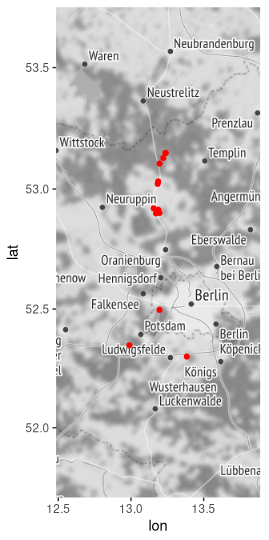
Map of collection sites