Freie Universität Berlin

Selecting what my be pedagogically valuable

Currently, I am teaching a lab course on plant morphology and biodiversity. In order for my students to work on live plant material, I have spent a lot of time in the greenhouses of the Botanical Garden and Botanical Museum Berlin-Dahlem to select appropriate study objects. Here are some of the examples my students are working with.

Canarina canariensis (Campanulaceae) from the western Canary Islands

Canarina canariensis (L.) Vatke (Campanulaceae)

Solanum laxum (Solanaceae) from southeastern Brasil, northern Argentina, Uruguay and Paraguay

Solanum laxum Spreng. (Solanaceae)

Michael Grünstäudl (Hominidae) from Austria

Michael Grünstäudl (Hominidae)

Tricky at first, but immensely helpful.

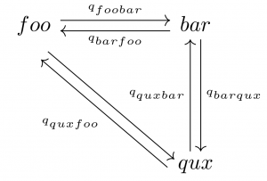
As I become more familiar with Latex, I realize how efficient this markup language is for generating publication-quality diagrams and figures. For a commutative diagram displaying the transition rates of plant leaf shapes, the following Latex code suffices to generate a clear and succinct graph.

Example of a communitative diagram in LaTeX

The early botanist catches the data

This week I collected some live plant material from our fantastic collection of water lilies for future sequencing of complete chloroplast genomes.

Nymphaea ampla DC.

Among the specimens collected was also the white water lily (Nymphaea ampla DC.), an enigmatic species that grows throughout Mesoamerica and that seems to have been an important component in Mayan rituals and of pharmacological use in their cultures (Bertol et al. 2004, J R Soc Med 97: 84–85).

Collecting Nymphaea ampla

Professional graphics require code

In order to visualize the location of oligonucleotide primers as well as structural rearrangements in plastid genomes, I wrote some Latex code.

When compiled, the above code generates the following image:

Schematic of Plastid Genome

A thank you goes to some fellow LaTeX Stack Exchange users, who assisted with the above code.

Easy if you know how.

We are living in a time of interconnectivity, and barely a day goes by when I don’t use the scripting language R in a more or less intricate pipeline. Often I have R call out to the interpreted programming language Python or the system shell to run a third-party executable (see the pipeline P2C2M as an example). In such situations it is essential that R and Python work together seamlessly.

To ensure inter-operability, it is important for each scripting language to call the correct version of the other. To do that, the setting of “default versions” is usually the way to go. But how do you set the default version of Python to be called by R?

In Linux:

In MacOS (assuming that your Python version of choice resides in /usr/local/bin/):

Upon setting the default version as shown above, it is important that you re-compile the R package with which you call Python (e.g., rPython) from source and re-install it.

Thanks go to my colleague Katie E. for sharing the above strategy necessary under MacOS.

R shell vs. RStudio

NOTE: This blog post originally appeared on 12-Nov-2014 on the blog I kept when I was a postdoctoral researcher at the Ohio State University. I am reposting it here because several people have asked me about this very topic lately.

On several occasions I have wondered which criterion the R package rPython employs to set the version of Python it interacts with. According to the installation file of rPython, “[b]y default, the package will be installed using the Python version given by $ python –version”. That seemed to be only part of the story, I thought, since my Linux system has Python 2.7.8 set as the default Python version, yet installations of the package via RStudio resulted in Python 3.4.1 being utilized by rPython:

What eluded me, however, was to evaluate if the command “python –version” would return Python 2.7.8, when run from RStudio, from where I usually install my R packages! Guess what: It does not.RStudio and the R shell invoke the bash shell differently, as evidenced by the following example:

In RStudio:

In R shell:

Hence, if I wish to have rPython interact with Python 2.7.8, I must install the package from the R shell.

… means attending lots of conferences, committees and seminars.

Sometimes it feels like I am more often in a suit than a lab coat.

Introduction of Seminar – Fall 2015

Talk at Conference

How to call the anticodon?

Over the past few days I have been correcting genomic annotations using custom bash and Python code. One of the more interesting exercises has been the homogenization of the “product” tags for transfer RNAs, which provide information about the respective anticodon sequences.

In the majority of databases familiar to me, anticodons are sometimes indicated by their DNA  (e.g., transfer RNA-Ile (GAT)), sometimes by their RNA sequence (e.g., transfer RNA-Ile (GAU)). I have yet to see a rule as to which version ought to be used.

In order to homogenize the spelling, I wrote a few lines of bash code. Interestingly, this coding problem is not a sed one-liner, but requires some intricate awk command (please see this Stackoverflow discussion for details).

Here is the solution I eventually adopted:

A brief, preliminary evaluation

For the revision of a new manuscript, I needed to generate a figure, in which a phylogenetic tree is plotted over a geographic map. The tips of the tree shall hereby point to the distribution area of the taxa they represent on the underlying map.

Lucky for me, Rod Page has recently published a small script, which plots the tips of a phylogenetic tree (stored in nexus-format) to latitude and longitude coordinates, which are saved as a geographic character alongside the tree.

php make_html.php MyTree.tre > MyTree.geojson

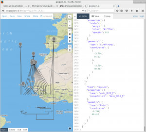
Upon running the script, I loaded the resulting geojson-file into the online tool geojson.io in order to evaluate the validity of the above-mentioned script. From the looks of it, this script does what it is supposed to do.

Screenshot geojson.io

In order to adjust line colour and thickness, I loaded the geojson-file into R using the rgdal library and plotted the results.

In summary, my first impression of this mapping procedure is quite positive.

Tree file format conversion for the efficient

Today, I needed to convert a series of phylogenetic trees, which were stored in the common nexus format, into newick format. In order to do this efficiently, I wrote the following one-liner.

Change into a directory containing your nexus-formatted tree files, then enter in your bash shell:

R -e 'require(ape); for (f in list.files(path=".", pattern="*.trees")) {write.tree(read.nexus(f), paste(f, "phy", sep="."))}'