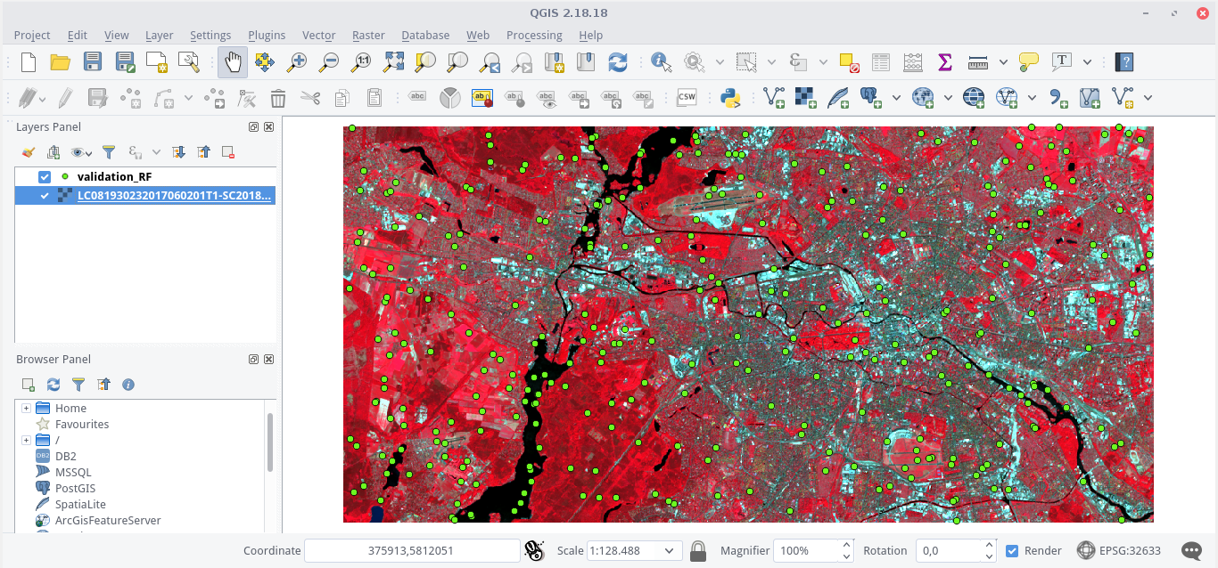
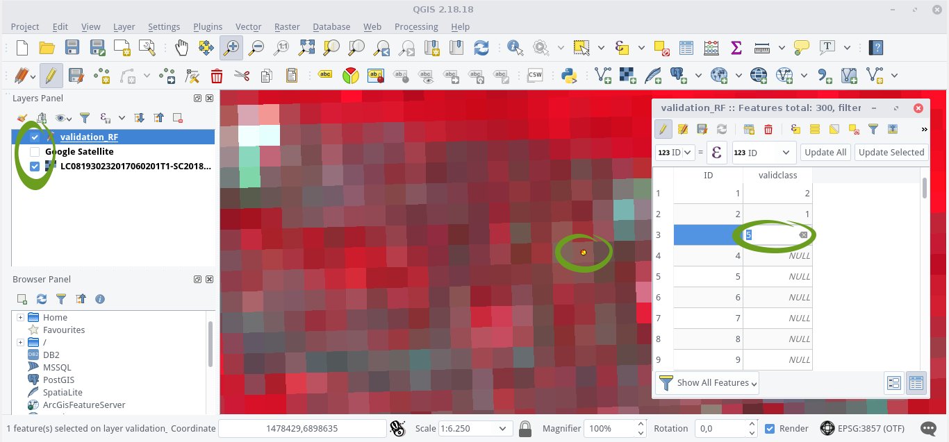
Open QGIS and import your initial image dataset (Landsat 8 scene) and the newly created point shapefile validation_RF.shp containing the test samples from the previous section. Display the image data using a RGB composite of your choice (see section Visualization in QGIS). A good, high-contrast presentation makes it easier to interpret the scene during validation:
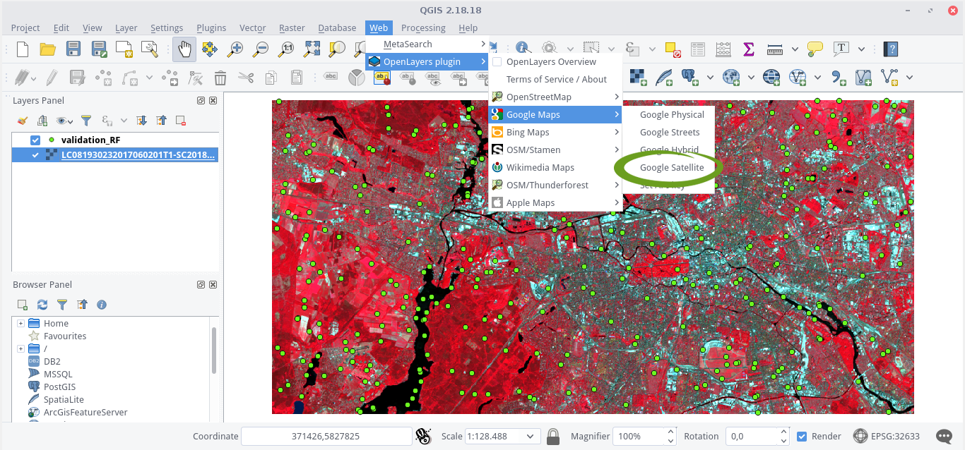
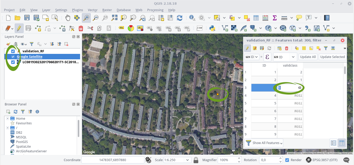
For visual support, we also want to look at the high-resolution information provided by Google Maps. Starting from the main menu of QGIS, navigate via Web > OpenLayers Plugin > Google Maps > Google Satellite to the satellite data from Google:
If you do not use our VM, you must first install the OpenLayers Plugin manually. See this guide to learn how to install a plugin.
Your data may look slightly rotated after the import of external Google Maps imagery. This is because the Google Maps data are subject to a different projection and they can not be reprojected on-the-fly. Because of this, your data will be temporarily adjusted so that everything is on top of each other.
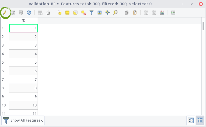
Right click your point shapefile (“validation_RF.shp”) and choose “Open Attribute Table”. Enable the editing features by pressing the pencil in the toolbar of the attribute table:
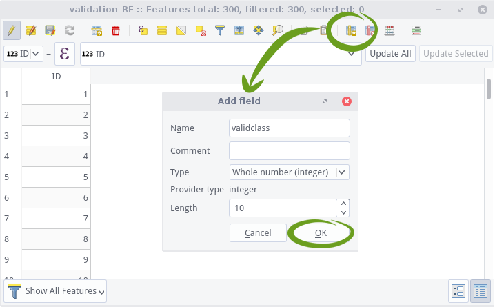
Now press the “new field” button ![]() in the toolbar to add a new column to the attribute table into which we will write the correct class labels. We just want to enter the number for the corresponding class, instead of typing the complete class names every time. So we need an integer column, which we call “validclass”. Copy the following settings and confirm with OK:
in the toolbar to add a new column to the attribute table into which we will write the correct class labels. We just want to enter the number for the corresponding class, instead of typing the complete class names every time. So we need an integer column, which we call “validclass”. Copy the following settings and confirm with OK:
Reminder: You wonder what numbers represent which class? Look again at section Prepare Samples in R. Starting from our training polygon shapefile, we were able to display the individual class labels and the corresponding class IDs in the following step. The order results according to the alphabetical sorting of the class names:
levels(as.factor(shp$classes))
## [1] "baresoil"  "forest"    "grassland" "urban_hd"  "urban_ld"  "water"

for (i in 1:length(unique(shp$classes))) {cat(paste0(i, " ", levels(as.factor(shp$classes))[i]), sep="\n")}
## 1 baresoil
## 2 forest
## 3 grassland
## 4 urban_hd
## 5 urban_ld
## 6 water
Write down the classification key! A wrong labeling of the points would be fatal for your validation statistics!
If the class IDs are finally known, you can start:
Zoom to a scale level that allows you to differentiate your target classes in Google Earth. Then click on the left part of a line in the attribute table to highlight/select it. Once selected, press the icon “Zoom to selected Features” in the toolbar or simply Control+J on your keyboard to automatically navigate to the respective point in the Map View:
Use both your initial dataset (Landsat 8) and any high-resolution information (Google Maps) to decide which class the pixel that contains the point belongs to.


