Landsat 8 ships as a tar-archived file with the spectral bands as individual georeferenced tif images. We want to stack these images into a single geotiff-file, i.e., into a so-called raster stack. Afterwards, it is much easier to work with such a raster stack. While this could also be done in QGIS, we will use R for this preprocessing, because it is easier to automate things this way. This results in the following intermediate steps we have to check off:

unzip your downloaded L8 files
put together the spectral band files of your choice into a rasterstack
save this rasterstack to your hard drive
(optional) delete all redundant data
(optional) create pyramid layers for a better visualization in QGIS

We will practice everything exemplarily on the basis of a single L8 Level-2 data set. There will be an exhaustive explanation for each line of code. Based on that we will develop a script that will automatically do everything for you in the future.

Prerequisite

The following content requires that you have either successfully downloaded some Landsat 8 scenes as part of the Download Section Exercise, or that you have acquired some datasets from the USGS EarthExplorer by your own. If this is not the case, look into the chapter Landsat / Earthexplorer!

Done? – Then start R-Studio now!

Preprocess a single dataset

We recommend writing the following code in the script window of R-Studio and executing it from there (see chapter R-Studio).
The example below assumes that you have one or more Landsat 8 scenes in a “landsatdata”-folder located in the exchange folder of your VM. Otherwise, adjust the folder according to your data!

We will use the raster library to write a raster file later. Additional libraries should always be loaded first, using the function library():

library(raster)
## Loading required package: sp

A few libraries make use of other libraries. So does the raster library with the sp-package, which will be loaded automatically.

Then define the Landsat 8 product of your choice with its entire file path and save it as the string variable product:

product <- "/media/sf_exchange/landsatdata/LC081930232017060201T1-SC20180613160412.tar.gz"

file.exists(product)
## [1] TRUE

NOTE: this is just an example – you have to change the file and its path according to your own settings!
You can use the function file.exists() to check whether the file can be found on your system or not. If it returns FALSE, make sure you did not mess up the file name.

We want to unpack the file into a folder with the same name as the file. The character variable product already contains the full name of the Landsat scene. We just have to get rid of the suffix “.tar.gz”. Therefore we can use the function substr() to delete the last seven characters (=”.tar.gz”) of the string:

productname <- substr(product, 1, nchar(product) - 7) 

productname
## [1] "/media/sf_exchange/landsatdata/LC081930232017060201T1-SC20180613160412"

The substring function substr() accepts three arguments here: a string (the entire file path with the suffix), and two integer values – one for a start (“1” = start with the first character) and one for a stop position within the given string. In order to define the stop position, we need to count the number of all characters of the file path via nchar(product) (which is 77 in our case) and substract 7.

Unzip the Landsat product using the untar() method and define the directory to which all data will be extracted by setting the argument exdir = productname:

untar(product, exdir = productname)

You should notice a new folder being created next to your initial data product. This could take a short moment. During processing, a red exclamation point can be seen in the upper right corner of the console window. NOTE: If this step fails, your data is corrupt. In this case, you will need to download the file again because something went wrong during data transfer.
After unpacking is complete, we want to have a look in the newly extracted folder and save the file names of all files in this folder into a vector productfiles using the function list.files. By providing the argument full.names = TRUE, the full paths are returned for each file:

productfiles <- list.files(productname, full.names = TRUE)

productfiles
##  [1] "/media/sf_exchange/landsatdata/LC081930232017060201T1-SC20180613160412/LC08_L1TP_193023_20170602_20170615_01_T1_ANG.txt"       
##  [2] "/media/sf_exchange/landsatdata/LC081930232017060201T1-SC20180613160412/LC08_L1TP_193023_20170602_20170615_01_T1_MTL.txt"       
##  [3] "/media/sf_exchange/landsatdata/LC081930232017060201T1-SC20180613160412/LC08_L1TP_193023_20170602_20170615_01_T1_pixel_qa.tif"  
##  [4] "/media/sf_exchange/landsatdata/LC081930232017060201T1-SC20180613160412/LC08_L1TP_193023_20170602_20170615_01_T1_radsat_qa.tif" 
##  [5] "/media/sf_exchange/landsatdata/LC081930232017060201T1-SC20180613160412/LC08_L1TP_193023_20170602_20170615_01_T1_sr_aerosol.tif"
##  [6] "/media/sf_exchange/landsatdata/LC081930232017060201T1-SC20180613160412/LC08_L1TP_193023_20170602_20170615_01_T1_sr_band1.tif"  
##  [7] "/media/sf_exchange/landsatdata/LC081930232017060201T1-SC20180613160412/LC08_L1TP_193023_20170602_20170615_01_T1_sr_band2.tif"  
##  [8] "/media/sf_exchange/landsatdata/LC081930232017060201T1-SC20180613160412/LC08_L1TP_193023_20170602_20170615_01_T1_sr_band3.tif"  
##  [9] "/media/sf_exchange/landsatdata/LC081930232017060201T1-SC20180613160412/LC08_L1TP_193023_20170602_20170615_01_T1_sr_band4.tif"  
## [10] "/media/sf_exchange/landsatdata/LC081930232017060201T1-SC20180613160412/LC08_L1TP_193023_20170602_20170615_01_T1_sr_band5.tif"  
## [11] "/media/sf_exchange/landsatdata/LC081930232017060201T1-SC20180613160412/LC08_L1TP_193023_20170602_20170615_01_T1_sr_band6.tif"  
## [12] "/media/sf_exchange/landsatdata/LC081930232017060201T1-SC20180613160412/LC08_L1TP_193023_20170602_20170615_01_T1_sr_band7.tif"  
## [13] "/media/sf_exchange/landsatdata/LC081930232017060201T1-SC20180613160412/LC08_L1TP_193023_20170602_20170615_01_T1.xml"

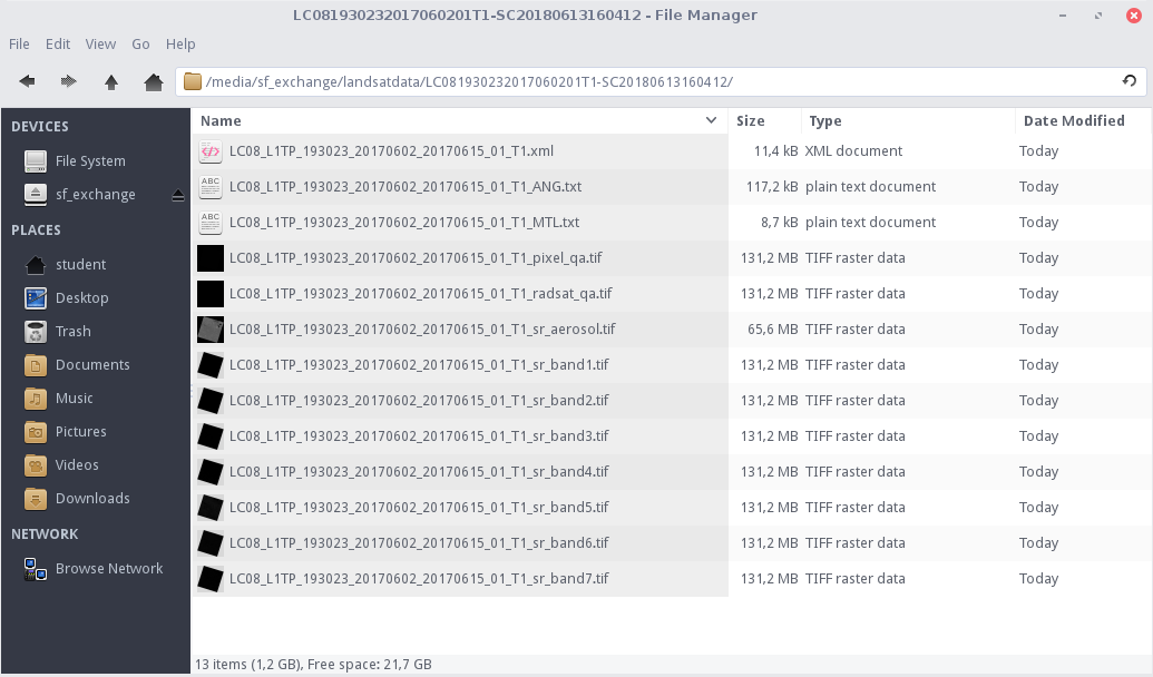
These are all 13 files that come with a Level-2 product (see Landsat 8 for more information). As a double check, you can have a look at the identical files in your file explorer:

Now we want to select all the spectral bands that we want to put into our new data stack. Have a deeper look at the files in productfiles. The files are named after the corresponding spectral channels at the end of the file name, e.g., “band1”, “band2”, and so on. We use these terms to extract the bands by utilizing the grep() function. The following code looks a little bloated. Maybe it is. But he gives you the freedom to exclude individual bands that you may not need. NOTE: This is an example of level 2 data. Landsat Level-1 scenes potentially have 11 channels. In the case of Level 1 data, you could easily enter the remaining lines here.

bands <- c(grep('band1', productfiles, value=TRUE),
           grep('band2', productfiles, value=TRUE),
           grep('band3', productfiles, value=TRUE),
           grep('band4', productfiles, value=TRUE),
           grep('band5', productfiles, value=TRUE),
           grep('band6', productfiles, value=TRUE),
           grep('band7', productfiles, value=TRUE)
           ) 

bands
## [1] "/media/sf_exchange/landsatdata/LC081930232017060201T1-SC20180613160412/LC08_L1TP_193023_20170602_20170615_01_T1_sr_band1.tif"
## [2] "/media/sf_exchange/landsatdata/LC081930232017060201T1-SC20180613160412/LC08_L1TP_193023_20170602_20170615_01_T1_sr_band2.tif"
## [3] "/media/sf_exchange/landsatdata/LC081930232017060201T1-SC20180613160412/LC08_L1TP_193023_20170602_20170615_01_T1_sr_band3.tif"
## [4] "/media/sf_exchange/landsatdata/LC081930232017060201T1-SC20180613160412/LC08_L1TP_193023_20170602_20170615_01_T1_sr_band4.tif"
## [5] "/media/sf_exchange/landsatdata/LC081930232017060201T1-SC20180613160412/LC08_L1TP_193023_20170602_20170615_01_T1_sr_band5.tif"
## [6] "/media/sf_exchange/landsatdata/LC081930232017060201T1-SC20180613160412/LC08_L1TP_193023_20170602_20170615_01_T1_sr_band6.tif"
## [7] "/media/sf_exchange/landsatdata/LC081930232017060201T1-SC20180613160412/LC08_L1TP_193023_20170602_20170615_01_T1_sr_band7.tif"

The grep() function searches for the string, which is given as the first argument, e.g., ‘band1’, in the vector of strings (2nd argument). Normally, when the function finds a match, it only returns the position of this find in the vector productfiles. By setting the argument value=TRUE we can write out the content of the vector at the respective position instead. By doing so, we create an vector bands containing all file paths via the standard combine-function c().

Now we can create a rasterstack based on the vector of bands in the variable bands. In order to do so, we use the function stack(), which is part of the raster-library we loaded in the beginning! This rasterstack function creates a rasterstack object based on a list of filenames. You will learn more about the beauty of rasterstacks in the chapter Visualization.

rasterstack <- stack( bands )

We can save this rasterstack and store it on your hard drive via writeRaster:

writeRaster(rasterstack, 
            paste0(productname, ".tif"), 
            format = "GTiff",
            overwrite = TRUE
            )

The writerRaster fuction is a powerful tool, which is also provided by the raster package. In line 1 we set our rasterstack object as the first argument. In line 2 we define the output name of the new file we will create. To do this, just add the suffix “.tif” to our filename using the handy function paste0, which just put all the strings together to one string. Line 3 explicitly defines the output format “GTiff”. How should I know this string “GTiff”, you ask? These strings are fixed by the function and are also listed for other data formats in the raster documentation on page 220. The fourth argument in line 4 only gives the authority to overwrite existing files.

DONE! A new file containing all spectral bands is now written directly next to the initial packed file you downloaded!

There are still two useful additional things left to do:
First, we can now delete the folder we created by uncompressing your Landsat data because it is no longer needed. So, if you want to save disk space, use the command unlink() to simply delete the folder. By setting the argument recursive=TRUE, all files within the folder will be deleted:

unlink(productname, recursive=TRUE)

Second, it is advisable to create so-called pyramid layers for each Landsat dataset. Pyramid layers are used to improve performance. They are a downsampled version of the original raster and speed up the display of raster data by retrieving only the data at a specified resolution that is required for the display. We can automatically create them by using the Geospatial Data Abstraction Library (GDAL). Initially, GDAL has nothing to do with R, but it can be operated via R using rgdal. However, we use the standalone installation of GDAL at this point, or more precisely, the function gdaladdo. If you do not use our VM, you have to install GDAL on your machine first. We build the appropriate command to run gdaladdo using paste0() and pass that command to the system() function. The system() function executes a command exactly as if you entered it yourself in the command window of Linux. Try it!

makeOVR <- paste0("gdaladdo -ro ", productname, ".tif 2 4 8 16")

makeOVR
## [1] "gdaladdo -ro /media/sf_exchange/landsatdata/LC081930232017060201T1-SC20180613160412.tif 2 4 8 16"

system( makeOVR )

Run the code and you will create a .ovr-file next to your .tif-file. This ovr-file holds the pyramid information, which will prove useful later in QGIS.

Phew! This was A LOT of (explanatory) text by now. Fortunately, the code is actually much shorter! Here is the complete code for preprocessing one exemplary L8 Level-2 file:

library(raster)

product <- "/media/sf_exchange/landsatdata/LC081930232017060201T1-SC20180613160412.tar.gz"

productname <- substr(product, 1, nchar(product) - 7) 

untar(product, exdir = productname)

productfiles <- list.files(productname, full.names = TRUE)

bands <- c(grep('band1', productfiles, value=TRUE),
           grep('band2', productfiles, value=TRUE),
           grep('band3', productfiles, value=TRUE),
           grep('band4', productfiles, value=TRUE),
           grep('band5', productfiles, value=TRUE),
           grep('band6', productfiles, value=TRUE),
           grep('band7', productfiles, value=TRUE)
           ) 

rasterstack <- stack( bands )

writeRaster(rasterstack, 
            paste0(productname, ".tif"), 
            format = "GTiff",
            overwrite = TRUE
            )

unlink(productname, recursive=TRUE)

makeOVR <- paste0("gdaladdo -ro ", productname, ".tif 2 4 8 16")
system( makeOVR )

Learn how to automate things for many datasets in the next section!

Freie Universität Berlin

Landsat 8 Preprocessing

Prerequisite

Preprocess a single dataset