Visualize in R

Also for this chapter it is a requirement that you own at least one Landsat 8 scene. We will visualize the Landsat 8 Level-2 scene (ID: LC08_L1TP_193023_20170602_20170615_01_T1) in R in this section, which you may have already downloaded in our EarthExplorer download exercise. You can download the preprocessed file here.

When you are ready, open R-Studio.

We need the raster package again, so import it into your current working session first:

library(raster)
## Loading required package: sp

The raster package offers various structures for importing data, depending on how the image data precedes:

layer() – one file, one band
stack() – multiple files, multiple bands
brick() – one file, multiple bands

During preprocessing (chapter Preprocess), we saved the individual bands of the Landsat 8 scenes in a single geotiff-container. So we created one file with several bands, so we need the brick() function for an import into R:

path <- "/media/sf_exchange/landsatdata/LC081930232017060201T1-SC20180613160412.tif"

img <- brick(path)

img
## class       : RasterBrick 
## dimensions  : 8141, 8051, 65543191, 7  (nrow, ncol, ncell, nlayers)
## resolution  : 30, 30  (x, y)
## extent      : 278085, 519615, 5762085, 6006315  (xmin, xmax, ymin, ymax)
## coord. ref. : +proj=utm +zone=33 +datum=WGS84 +units=m +no_defs +ellps=WGS84 +towgs84=0,0,0 
## data source : /media/sf_exchange/landsatdata/LC081930232017060201T1-SC20180613160412.tif 
## names       : LC0819302//13160412.1, LC0819302//13160412.2, LC0819302//13160412.3, LC0819302//13160412.4, LC0819302//13160412.5, LC0819302//13160412.6, LC0819302//13160412.7 
## min values  :            -3.400e+38,            -2.000e+03,            -1.685e+03,            -1.384e+03,            -2.720e+02,            -1.060e+02,            -6.500e+01 
## max values  :                 13333,                 13643,                 14703,                 14674,                 14331,                 15137,                 15638

By calling the object img in line 5, the most important metadata can be viewed, e.g., raster dimensions, geometric resolution, geographical extent, coordinate system, file path, as well as minimum and maximum digital numbers per band. This completes the import of the L8 image as a RasterBrick object into R.

We can now plot the image data. The plotRGB() function is a convenient way to visualize different RGB composites. Check out the help for this feature in R-Studio by running ?plotRGB! The function has three arguments called r =, g =, and b =, which define the three layers to be used for the RGB slots in a RasterBrick or Rasterstack.
If we just want to visualize one band (singleband visualization), we will fill all three slots with the same band, e.g. the green band:

plotRGB(img,
        r = 3, g = 3, b = 3,
        stretch = "lin"
        )

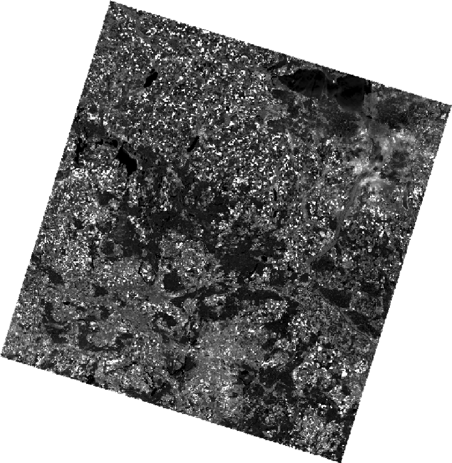
The stretch argument in line 3 was set to “lin” in order to perform a minimum-maximum contrast stretching to increase the contrast of the image, as described here.
We can also do a spatial subsetting here by specifying an “Extent”-object using the ext = argument:

plotRGB(img,
        r = 3, g = 3, b = 3,
        stretch = "lin",
        ext = extent(369800, 400700, 5812400, 5827500)
        )

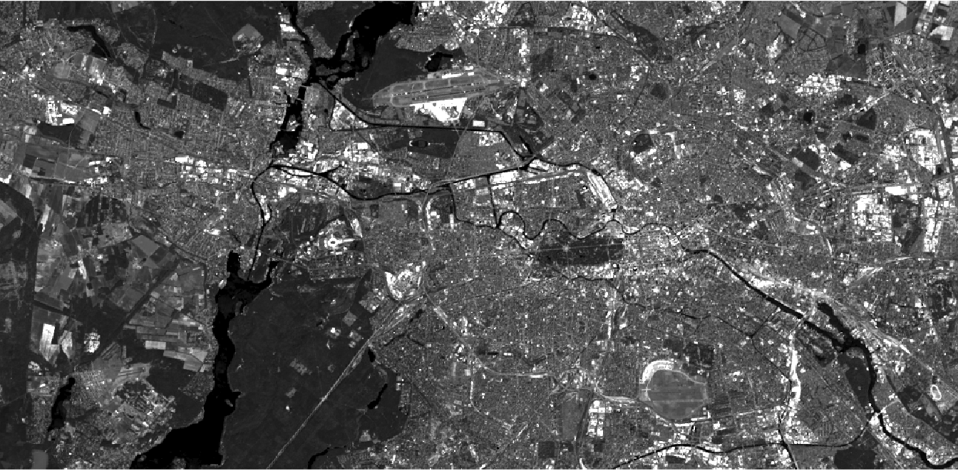
Objects of class “Extent” are used to define the spatial extent. The four specified arguments are UTM coordinates for (min x, max x, min y, max y). You can set those UTM coordinates arbitrarily and get them, for example, by reading them from QGIS or Google Maps.

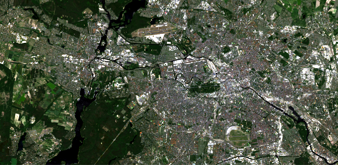
By defining different bands for the RGB slots, we can, just as in QGIS, create all imaginable RGB composites:

plotRGB(img,
        r = 4, g = 3, b = 2,
        stretch = "lin",
        ext = extent(369800, 400700, 5812400, 5827500)
        )

Make your spatial subset permament by writing the trimmed image as a new file to your hard drive with writeRaster. This is especially useful if you want to test a classification workflow: small data sets will cheer up your work in QGIS, in R, as well as in all other software solutions.

img.subset <- crop(img, extent(369800, 400700, 5812400, 5827500) )

writeRaster(img.subset,
            filename = "/media/sf_exchange/landsatdata/LC081930232017060201T1-SC20180613160412_subset.tif",
            format = "GTiff",
            overwrite = TRUE
            )

Of course, it is also possible to examine the underlying data distribution in more detail. Therefore, we can look at a histogram of a specific band with the function hist():

green <- img.subset[[3]]

hist(green,
     breaks = 200,
     xlim = c(0, 2000),
     ylim = c(0, 120000),
     xlab = "band 3 reflectance value [DN * 0.01]",
     ylab = "frequency",
     main = "histogram L8 band 3 (green)"
     )

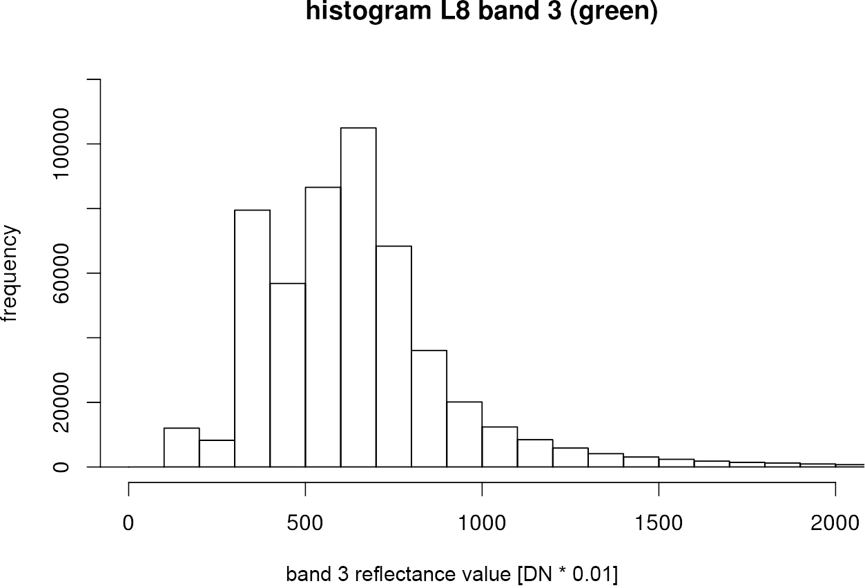
The breaksargument in line is assigned with a single number giving the number of cells for the histogram. So with more breaks, the bars in the histogram become narrower. With xlim =and ylim =you can narrow the x axis and y axis to a certain range.

NEXT
ANALYSE