The concept of Support Vector Machines (SVM) was introduced in the context of pattern recognition and machine learning in 1979 by Vapnik & Chervonenkis. A SVM is a powerful tool for highdimensional, linear and non-linear data science problems. It is always a good choice to consider a SVM for classification and regression tasks due to its high customizability and settings options. However, the search procedure for critical parameter is more complex compared to the RF.
Let us have a look at the basic concepts of a supervised SVM implementation for a classification task.
Basic Concept
Consider a set of labelled training samples \(X\), e.g., pixels of an RS image. Each sample is a single vector in the feature space, e.g., one grey scale value for each of the 11 spectral bands of a Landsat 8 scene gives a vector with dimensions \(1\times8\). The concept of a SVM is based on an optimal linear separating hyperplane that is fitted to the training samples of two classes within this multidimensional feature space. Thereby, the optimization problem that has to be solved is aiming at a maximization of the margins between this hyperplane and the closest training samples, the so-called and name giving Support Vectors. Only those Support Vectors are needed to describe the hyperplane mathematically exact, vectors farther from the hyperplane remain hidden. The following figure shows a hyperplane separating two classes in two-dimensional space, e.g. Band 3 on the x-axis and Band 4 on the y-axis:
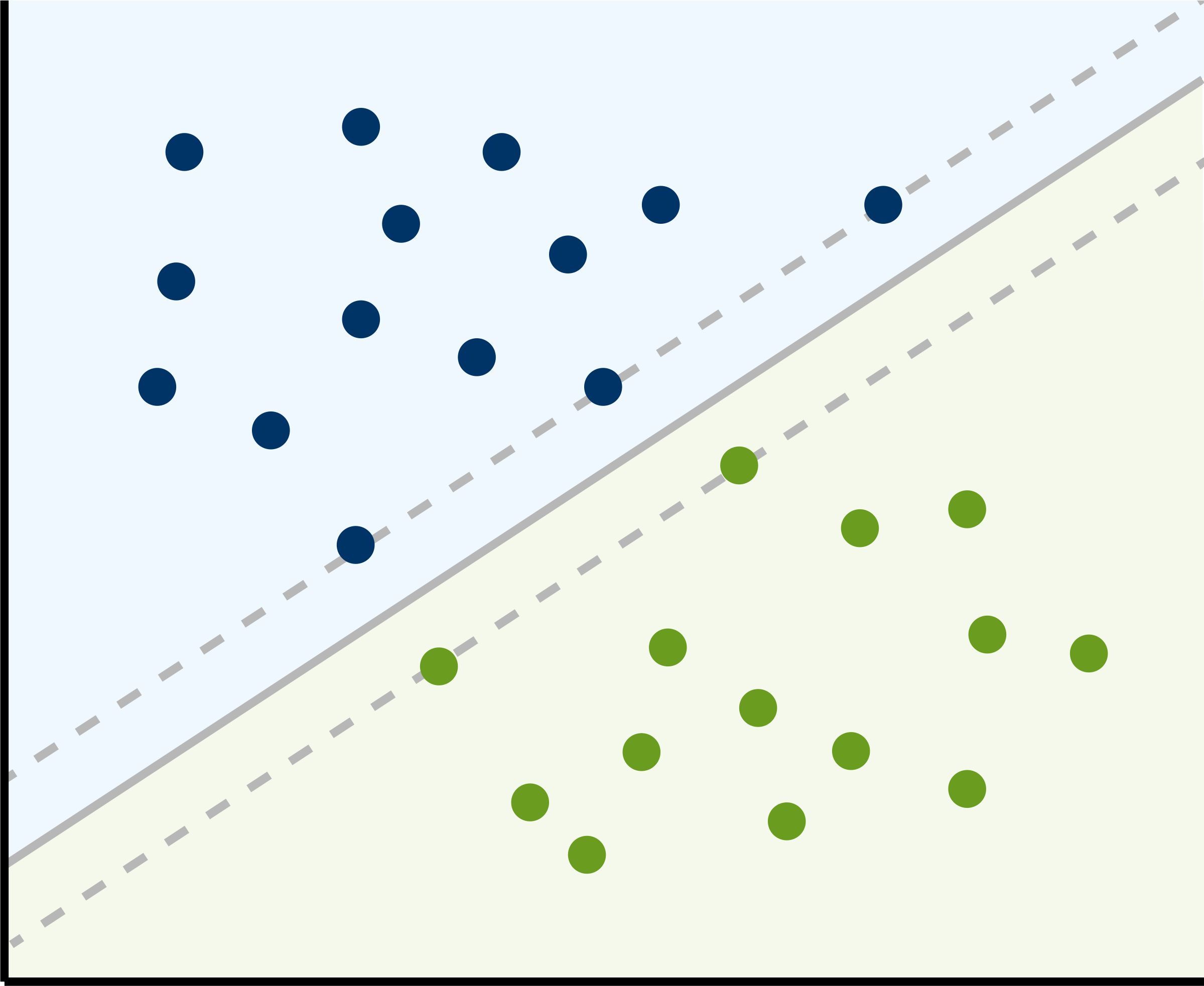
This wide and empty border area surrounding the hyperplane should ensure that new vectors, which are not in our training dataset, i.e., pixels in RS imagery, will be classified as reliably as possible in a later prediction process.
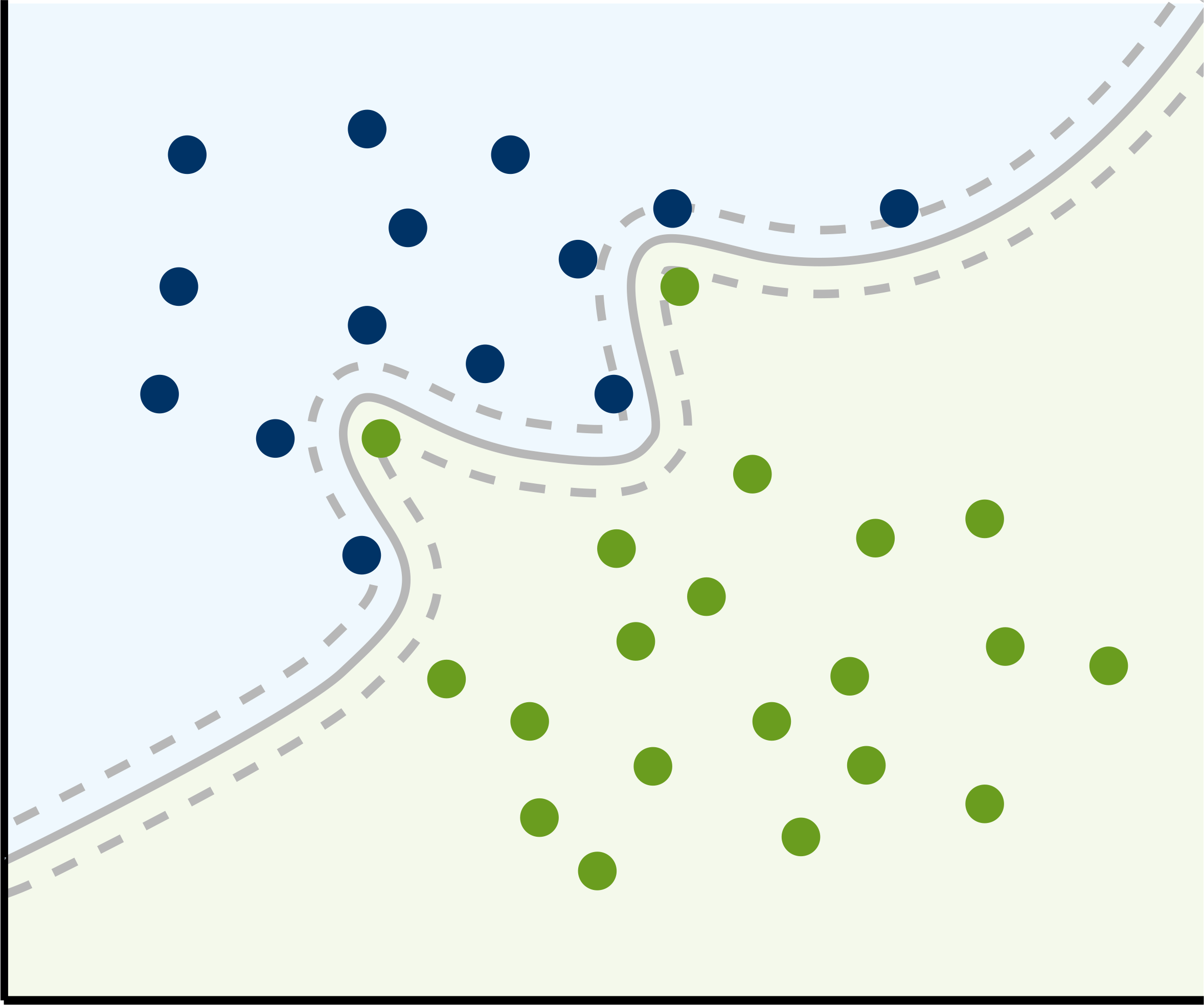
Ok, the classification problem in the figure above is very easy to solve linearly. However, the condition of linear separability is generally not met in real-life data. In the case of non-linear separable samples, the SVM needs a so-called kernel. A kernel is actually a function, which maps the data into a higher dimensional space where the data is separable. There are several of these kernels, such as linear, polynomial, radial basis and sigmoid kernels, with the radial basis function (RBF) kernel most commonly used for non-linear problems. In doing so, even the most nested training samples become linear separable and the hyperplane can be determined. After a transformation back into the initial lower-dimensional space, this linear hyperplane can become a non-linear or even un-connected hypersurface:
In the context of Remote Sensing, binary classification problems are not common. There are several approaches to solve multi-class problems, the most frequently used approach is the one-against-one rule, which is also implemented in the e1071 package we use in the next section. According to this one-against-one approach, a binary classifier is trained for each pair-wise class combination, and the most frequently assigned class label is assigned in the end.
Common Parameters
Regularisation parameter \(C\): As the hyperplane can be of arbitrary dimensionality, it could be fitted perfectly to match the training dataset. However, this would result in extreme overfitting. To regularisation parameter C allows the SVM to misclassify individual samples, but at the same time punish them. Large C values cause the hyperplane margin to shrink, which may help to increase the amount of correctly classified samples. Conversely, a small C value will result in a larger-margin hyperplane, leading to lower punishments and maybe more misclassified samples.
Kernel parameter gamma \(\gamma\): This parameter defines how far the influence of a single training sample reaches, i.e., its radius of influence. Low values mean “far”, and high values mean “close”. The model performance is quite sensitive to this parameter: when gamma is too large, the radii of influence of the SVs are too small and only affect the SVs itself, making the regularisation with C impossible and thus lead to overfitting. When gamma is too small, the model is too constrained and may not be capable to capture the complexity of our training dataset.
Parameter epsilon \(\varepsilon\) (only in regressions): The epsilon parameter is an additional value of tolerance where no penalty is given to errors. The larger epsilon is, the larger errors you allow in your model. When epsilon is zero, all errors will be penalized.