We want to put the training samples created in the previous section in the form of a data frame – which most classifiers in R can handle easily (especially our RF and SVM algorithms). You can download the training_data shapefile here. For this task, we again take advantage of the powerful raster package. The complete code is shown below and a more detailed description is given afterwards.
# import raster package
library(raster)

# import image (img) and shapefile (shp)
setwd("/media/sf_exchange/landsatdata/")
img <- brick("LC081930232017060201T1-SC20180613160412_subset.tif")
shp <- shapefile("training_data.shp")

# extract samples with class labels and put them all together in a dataframe
names(img) <- c("b1", "b2", "b3", "b4", "b5", "b6", "b7")
smp <- extract(img, shp, df = TRUE)
smp$cl <- as.factor( shp$classes[ match(smp$ID, seq(nrow(shp)) ) ] )
smp <- smp[-1]
In-depth Guide
In order to use functionalities of the raster package, load it into your current session via library(). If you do not use our VM, you must first download and install the packages with install.packages():
#install.packages("raster")
library(raster)
Next: set your working directory, in which all your image and shapefile data is stored by giving a character (do not forget the quotation marks ” “) variable to setwd(). Check your path with getwd() and the stored files in it via dir():
setwd("/media/sf_exchange/landsatdata/")

getwd()
## [1] "/media/sf_exchange/landsatdata"

dir()
## [1] "LC081930232017060201T1-SC20180613160412_subset.tif"
## [2] "polygons_training.dbf"
## [3] "polygons_training.prj"
## [4] "polygons_training.qpj"
## [5] "polygons_training.shp"
## [6] "polygons_training.shx"
If you do not get your files listed, you have made a mistake in your work path – check again! Everything ready to go? Fine, then import your raster file as img and your shapefile as shp and have a look at them:
img <- brick("LC081930232017060201T1-SC20180613160412_subset.tif")
img
## class       : RasterBrick
## dimensions  : 504, 1030, 519120, 7  (nrow, ncol, ncell, nlayers)
## resolution  : 30, 30  (x, y)
## extent      : 369795, 400695, 5812395, 5827515  (xmin, xmax, ymin, ymax)
## coord. ref. : +proj=utm +zone=33 +datum=WGS84 +units=m +no_defs +ellps=WGS84 +towgs84=0,0,0
## data source : /media/sf_exchange/landsatdata/LC081930232017060201T1-SC20180613160412_subset.tif
## names       : LC0819302//2_subset.1, LC0819302//2_subset.2, LC0819302//2_subset.3, LC0819302//2_subset.4, LC0819302//2_subset.5, LC0819302//2_subset.6, LC0819302//2_subset.7
## min values  :                 -2000,                 -2000,                 -1502,                 -1384,                  -107,                   -72,                   -27
## max values  :                 13240,                 13539,                 14574,                 14549,                 14243,                 14896,                 15388

shp <- shapefile("training_data.shp")
shp
## class       : SpatialPolygonsDataFrame
## features    : 72
## extent      : 369802.9, 400028.9, 5812457, 5827504  (xmin, xmax, ymin, ymax)
## coord. ref. : +proj=utm +zone=33 +datum=WGS84 +units=m +no_defs +ellps=WGS84 +towgs84=0,0,0
## variables   : 1
## names       :  classes
## min values  : baresoil
## max values  :    water

compareCRS(shp, img)
## [1] TRUE
Both the brick() and shapefile() functions are provided by the raster package. As shown above, they create objects of the class RasterBrick and SpatialPolygonsDataFrame respectively. The L8 raster provides 7 bands, and our example shapefile 72 features, i.e., polygons. You can check whether the projections of the two datasets are identical or not by executing compareCRS(shp, img). If this is not the case (output equals FALSE), the raster package will automatically re-project your data on the fly later on. However, we recommend to adjust the projections manually in advance to prevent any future inaccuracies.
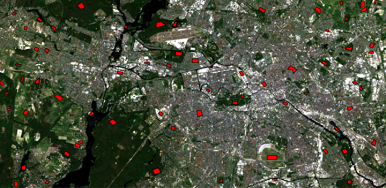
Plot your data to make sure everything is imported properly (check Visualize in R for an intro to plotting). With the argument add = TRUE in line 2 several data layers can be displayed one above the other:
plotRGB(img, r = 4, g = 3, b = 2, stretch = "lin")
plot(shp, col="red", add=TRUE)
If you followed this course in the previous section, your shapefile should provide an attribute called “classes”, which includes your target classes as strings, e.g., “water” or “urban”. We will later turn this column into the factor data type because classifiers can only work with integer values instead of words like “water” or “urban”. When converting to factors, strings are sorted alphabetically and numbered consecutively. In order to be able to read the classification image at the end, you should make a note of your classification key:
levels(as.factor(shp$classes))
## [1] "baresoil"  "forest"    "grassland" "urban_hd"  "urban_ld"  "water"

for (i in 1:length(unique(shp$classes))) {cat(paste0(i, " ", levels(as.factor(shp$classes))[i]), sep="\n")}
## 1 baresoil
## 2 forest
## 3 grassland
## 4 urban_hd
## 5 urban_ld
## 6 water
The levels() function combines all occurrences in a factor-formatted vector. In the example shown above, value 1 in our classification image will correspond to the baresoil class, value 2 to forest, value 3 to grassland, etc.
Optional: Let us take a look at the naming of the raster bands via the names() function. Those names can be quite bulky and cause problems in some illustrations when used as axis labels. You can easily rename it to something more concise by overriding the names with any string vector of the same length:
names(img)
## [1] "LC081930232017060201T1.SC20180613160412_subset.1"
## [2] "LC081930232017060201T1.SC20180613160412_subset.2"
## [3] "LC081930232017060201T1.SC20180613160412_subset.3"
## [4] "LC081930232017060201T1.SC20180613160412_subset.4"
## [5] "LC081930232017060201T1.SC20180613160412_subset.5"
## [6] "LC081930232017060201T1.SC20180613160412_subset.6"
## [7] "LC081930232017060201T1.SC20180613160412_subset.7"

names(img) <- c("b1", "b2", "b3", "b4", "b5", "b6", "b7")

names(img)
## [1] "b1" "b2" "b3" "b4" "b5" "b6" "b7"
Appropriate names for the input features are very helpful for orientation and readability. Of course you need to change the vector in line 10 according to your own input features.
Our goal is to extract the raster values (x), i.e., all input feature values, and the class values (y) of every single pixel within our training polygons and put all together in a data frame. This data frame can then be read by our classifier. We extract the raster values using the command extract() from the raster package. The argument df = TRUE guarantees that the output is a data frame:
smp <- extract(img, shp, df = TRUE)
It may take some (long) time for this function to complete depending on the spatial resolution of your raster data and the spatial area covered by your polygons. If you have your data stored on an SSD, the process is completed much faster. It may be advisable to save the resulting object to the hard drive save(smp , file = “smp .rda”) and load it from the hard disk if necessary load(file = “smp.rda”). On this way, the extract function does not have to be repeated again and again…
The data frame has as many rows as pixels could be extracted and as many columns as input features are given (in this example the spectral channels). In addition, smp also provides a column named “ID”, which holds the IDs of the former polygon for each pixel (each polygon is automatically assigned an ID). Furthermore, we also know which polygon, i.e., each ID, belongs to which class. Because of this, we can establish a relationship between the deposited ID of each pixel and the class using the match() function. We use this to add another column to our data query describing each class. Then we delete the ID column because we do not need it anymore:
smp$cl <- as.factor(shp$classes[match(smp$ID, seq(nrow(shp)))])
smp <- smp[-1]

summary(smp$cl)
##  baresoil    forest grassland  urban_hd  urban_ld     water
##       719      2074      1226      1284       969       763

str(smp)
## 'data.frame':    7035 obs. of  8 variables:
##  $ b1: num  192 179 189 159 171 164 173 184 144 150 ...
##  $ b2: num  229 203 221 179 194 188 192 208 166 165 ...
##  $ b3: num  321 233 272 188 203 196 208 254 178 177 ...
##  $ b4: num  204 130 164 97 116 108 119 150 83 80 ...
##  $ b5: num  161 156 173 125 146 138 146 166 107 104 ...
##  $ b6: num  100 93 109 63 82 71 82 104 51 46 ...
##  $ b7: num  72 68 81 40 56 51 59 74 32 30 ...
##  $ cl: Factor w/ 6 levels "baresoil","forest",..: 6 6 6 6 6 6 6 6 6 6 ...
Now you are ready to start training your classifier as described in the next sections!
Optional: If you only include spectral information in your classifier, as in our example, it is often helpful to plot the so-called spectral profiles, or z-profiles. Those represent the mean values of each class for the individual spectral bands. You can also represent other features, e.g., terrain height or precipitation, however, you must then pay attention to the value range in the presentation and possibly normalize the data at first. The magic here happens in the aggregate() command, which combines all the rows of the same class . ~ cl and calculates the arithmetic mean of those groups FUN = mean. This happens for all classes, in the cl column, where NA values are to be ignored via na.rm = TRUE. The rest of the functions in the following script are for visualization purposes only and include standard functions such as plot(), lines(), grid() and legend(). Use the help function for a detailed description of the arguments!
sp <- aggregate( . ~ cl, data = smp, FUN = mean, na.rm = TRUE )

# plot empty plot of a defined size
plot(0,
     ylim = c(min(sp[2:ncol(sp)]), max(sp[2:ncol(sp)])),
     xlim = c(1, ncol(smp)-1),
     type = 'n',
     xlab = "L8 bands",
     ylab = "reflectance [% * 100]"
     )

# define colors for class representation - one color per class necessary!
mycolors <- c("#fbf793", "#006601", "#bfe578", "#d00000", "#fa6700", "#6569ff")

# draw one line for each class
for (i in 1:nrow(sp)){
  lines(as.numeric(sp[i, -1]),
        lwd = 4,
        col = mycolors[i]
        )
  }

# add a grid
grid()

# add a legend
legend(as.character(sp$cl),
       x = "topleft",
       col = mycolors,
       lwd = 5,
       bty = "n"
       )
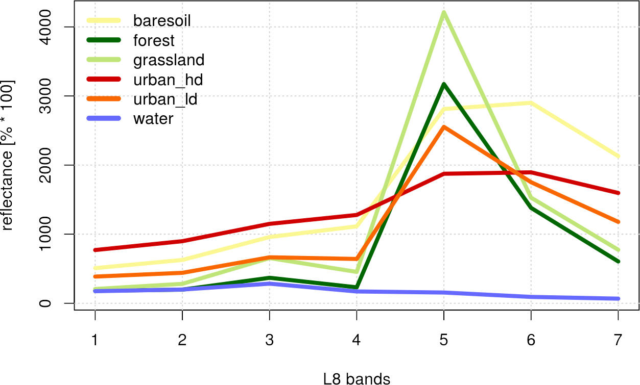
Note that the values represent only the arithmetic mean of the classes and do not allow any statement about the underlying distribution. However, such a z-profile plot helps to visually assess the separability of classes at the beginning.