There are some packages available containing the possibility to perform the standard RF algorthm described by Breiman (2001), e.g., in the caret, randomForest, ranger, xgboost, or randomForestSRC packages. However, we will use the package called “randomForest” because it is the most common and therefore best supported.
Below you can see a complete code implementation. While this is already executable with your input data, you should read the following comprehensive in-depth guide to understand the code in detail. Even better: You will learn how to generate numerous useful plots, which do great in each thesis!
# import packages
library(raster)
library(randomForest)

# import image (img) and shapefile (shp)
setwd("/media/sf_exchange/landsatdata/")
img <- brick("LC081930232017060201T1-SC20180613160412_subset.tif")
shp <- shapefile("training_data.shp")

# extract samples with class labels and put them all together in a dataframe
names(img) <- c("b1", "b2", "b3", "b4", "b5", "b6", "b7")
smp <- extract(img, shp, df = TRUE)
smp$cl <- as.factor( shp$classes[ match(smp$ID, seq(nrow(shp)) ) ] )
smp <- smp[-1]

# tune and train rf model
smp.size <- rep(min(summary(smp$cl)), nlevels(smp$cl))
rfmodel <- tuneRF(x = smp[-ncol(smp)],
                  y = smp$cl,
                  sampsize = smp.size,
                  strata = smp$cl,
                  ntree = 250,
                  importance = TRUE,
                  doBest = TRUE
                  )

# save rf model
save(rfmodel, file = "rfmodel.RData")

# predict image data with rf model
result <- predict(img,
                  rfmodel,
                  filename = "classification_RF.tif",
                  overwrite = TRUE
                  )
In-depth Guide
In order to be able to use the functions of the randomForest package, we must additionally load the library into the current session via library(). If you do not use our VM, you must first download and install the packages with install.packages():
#install.packages("raster")
#install.packages("randomForest")
library(raster)
library(randomForest)
First, it is necessary to process the training samples in the form of a data frame. The necessary steps are described in detail in the previous section.
names(img) <- c("b1", "b2", "b3", "b4", "b5", "b6", "b7")
smp <- extract(img, shp, df = TRUE)
smp$cl <- as.factor( shp$classes[ match(smp$ID, seq(nrow(shp)) ) ] )
smp <- smp[-1]
After that, you can identify the number of available training samples per class with summary(). There is often an imbalance in the number of those training pixels, i.e., one class is represented by a large number of pixels, while another class has very few samples:
summary(smp$cl)
##  baresoil    forest grassland  urban_hd  urban_ld     water
##       719      2074      1226      1284       969       763
This often leads to the problem that classifiers favor and overclass strongly-represented classes in the classification. However, the Random Forest Algorithm, as an ensemble classifier, provides an ideal solution to compensate for this imbalance. For each decision tree, we draw a bootstrap sample from the minority class (class with the fewest samples). Then, we randomly draw the same number of cases, with replacement, from all other classes. This technique is called down-sampling.
In our example this is the class baresoil with 719 samples. With the rep() function we form a vector where the length corresponds to the number of target classes. We will use this vector to tell the classifier how many samples it should randomly draw per class for each decision tree during training:
smp.size <- rep(min(summary(smp$cl)), nlevels(smp$cl))
smp.size
## [1] 719 719 719 719 719 719
The complete training takes place via just one function call of tuneRF()! This function automatically searches for the best parameter setting for mtry – the number of variables available for each tree node. So we just have to worry about ntree, i.e., the number of trees to grow. 250-1000 trees are usually sufficient. Basically, the more the better, but many trees will increase the calculation time. When tuneRF() is called, we need to specify the training samples as x, i.e., all columns of our smp dataframe except the last one, and the corresponding class labels as y, i.e. the last column of our smp dataframe called “cl”:
rfmodel <- tuneRF(x = smp[-ncol(smp)],
                  y = smp$cl,
                  sampsize = smp.size,
                  strata = smp$cl,
                  ntree = 250,
                  importance = TRUE,
                  doBest = TRUE
                  )
## mtry = 2  OOB error = 2.5%
## Searching left ...
## mtry = 1     OOB error = 2.54%
## -0.01704545 0.05
## Searching right ...
## mtry = 4     OOB error = 2.7%
## -0.07954545 0.05
In line 3, we pass our smp.size vector as argument the sampsize = to define how many samples it should draw per class, and strata = at line 4 defines the column which should use for this stratified sampling. The argument importance = in line 6 allows the subsequent assessment of the variable importance when set to TRUE. By setting the argument doBest to TRUE, the RF with the optimal mtry is output directly from the function.
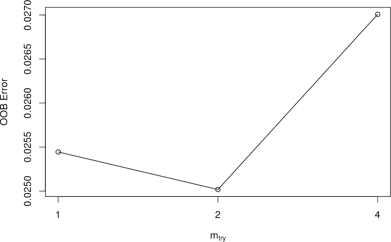
If you use tuneRF, you will automatically get a plot that will tell you the OOB errors in the dependency of different mtry settings. As mentioned, the feature automatically identifies the best mtry setting and uses this to generate the optimal RF.
When the model is created, we get some really useful information by executing the object name. First we get the command call with which we trained the model and the final number of variables tried at each split, i.e. the mtry parameter. Furthermore, we get an averaged out of bag (OOB) estimate, as well as a complete confusion matrix based on the training data! The column headers contain the classes of training pixels and the rows describe the corresponding classification. For a more detailed description of a confusion matrix, please refer to the chapter Validate Classifiers.
rfmodel
##
## Call:
##  randomForest(x = smp[-ncol(smp)], y = smp$cl, ntree = 300, mtry = mtry.opt,
##               strata = smp$cl, sampsize = smpsize, importance = TRUE)
##                Type of random forest: classification
##                      Number of trees: 300
## No. of variables tried at each split: 2
##
##         OOB estimate of  error rate: 2.52%
## Confusion matrix:
##           baresoil forest grassland urban_hd urban_ld water class.error
## baresoil       708      0         2        3        6     0 0.015299026
## forest           0   2060         2        0       11     1 0.006750241
## grassland        4      0      1220        0        2     0 0.004893964
## urban_hd        18      0         0     1204       62     0 0.062305296
## urban_ld         7     10         9       39      904     0 0.067079463
## water            0      0         0        1        0   762 0.001310616
Before we started the training procedure, we set the argument importance = true, which now allow us to have a look at the importance variable using the varImpPlot command:
varImpPlot(rfmodel)
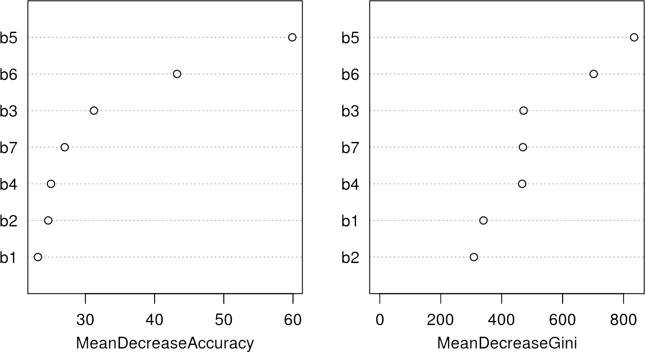
The variable importance shows the most significant or important features for the classification, which are band 5 and 6 in this case. For details of those metrics, please refer to the Random Forest Section. However, it is interesting to note that the most important bands also provide the largest spectral differences between the classes in the previous section.
Additionally, you can plot the RF model itself, which shows you the relationship between OOB Error and the number of trees used. We can color the lines by passing a vector of hex-colors whose length equals the number of classes + 1 – the first color is the average OOB line, which is also plotted automatically:
plot(rfmodel, col = c("#000000", "#fbf793", "#006601", "#bfe578", "#d00000", "#fa6700", "#6569ff"))
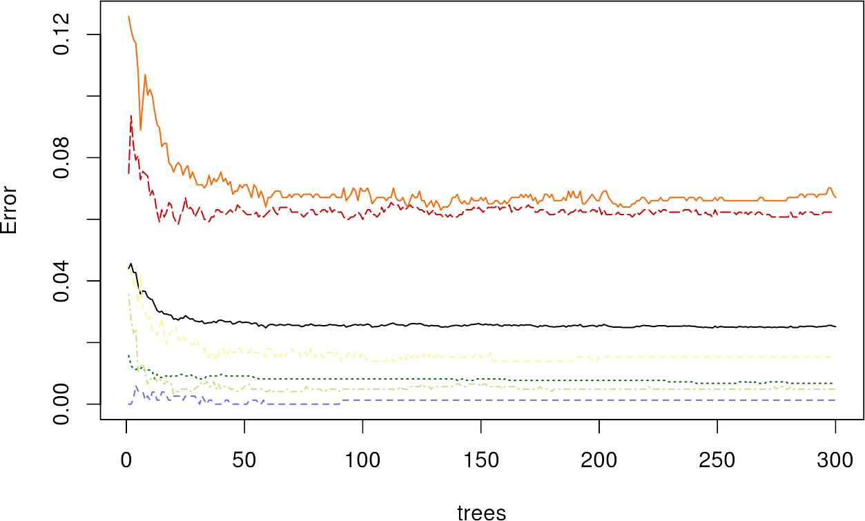
We can see a decrease in the error with increasing number of trees, where the urban classes have the highest OOB error values.
Save the model by using the save() function. This function saves the model object rfmodel to your working directory, so that you have it permanently stored on your hard drive. If needed, you can load it any time with load().
save(rfmodel, file = "rfmodel.RData")
#load("rfmodel.RData")
Since your model is now fully trained, you can use it to predict all the pixels in your image. The command method predict() takes a lot of work from you: It is recognized that there is an image which then passes through your Random Forest pixel by pixel. As with the training pixels, each image pixel is now individually classified and finally reassembled into your final classification image. Use the argument filename = to specify the name of your output map:
result <- predict(img,
                  rfmodel,
                  filename = "classification.tif",
                  overwrite = TRUE
                  )
Random Forest classification completed!
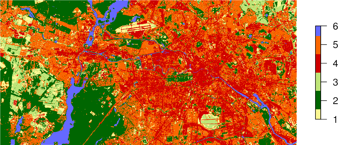
If you store the result of the predict() function in an object, e.g., result, you can plot the map using the standard plot command and passing this object:
plot(result,
     axes = FALSE,
     box = FALSE,
     col = c("#fbf793", # baresoil
             "#006601", # forest
             "#bfe578", # grassland
             "#d00000", # urban_hd
             "#fa6700", # urban_ld
             "#6569ff"  # water
             )
     )