This section provide a guide on how to create training areas in the form of polygons, which we save in a shapefile in QGIS. The process is very similar to collecting samples in ArcGIS/ ArcMAP, which you already know from our GIS seminars.

Collecting training areas is essential when working with supervised classifiers and significantly influences the classification outputs. You should make some preliminary considerations and approach the sampling very carefully! In the following, we will focus on the most important basics to consider.

Preliminary thoughts about sampling

Probably the most frequently asked questions are how many polygons should be created by class and and how big should they be?
– Good questions!

Unfortunately, those just can not be answered directly. The amount of training data you need, i.e., polygon count and size, depends both on the

• complexity of your classification problem (number and similarity of target classes, …) &
• complexity of your classification algorithm (number of parameters or weights, RF, SVM, ANN, ML, …).

Sampling data in machine learning is a science in itself, which is why there is a wealth of scientific publications about it (Curran & Williamson 1986, Figueroa et al. 2012) and even entire books (Marchetti et al. 2006, Hastie et al. 2017).

Fine, so far that is not much of a help…

To keep it very simple: You need a sample of your data that representatively describes the problem you want to solve. Keep in mind, a classifier learns a mathematical function, which maps input data (e.g., spectral bands) to output data (e.g., class labels). In order to achieve this, you should provide enough training data to capture the relationships between input and output. Training data will optimally meet the following requirements:

• independent of test data:
  A training dataset must be independent of the test dataset used for a validation, but can follow the same probability distribution. No training sample may be used to test (validate) the performance of the classifier! In the context of remote sensing data, it is also important that train and test data are spatially maximally distant to avoid spatial autocorrelation (Morans I).
• mostly identical distributed:
  Each target class should be equally represented in the training data set. Most datasets do not have an exactly equal number of instances in each class. Small differences often does not matter. However, if there is a strong imbalance, e.g., 90% of all training data represent class 1 and only 10% class 2, most algorithms very quickly overclassify the more-prevalent classes. Some simple options here: Collect more samples of the low-represented classes, use data augmentation to synthetically create new samples for under-represented classes, or use a under sampling method. The simplest under sampling method is to delete samples from the over-represented classes during classifier training. We will use this latter method for the RF and SVM implementations later on.
• representative for target classes:
  Training data should cover as many intra-class variations as possible, e.g., all spectral classes of a thematic target class, such as deciduous trees and conifers for the target class “forest”. Especially with more complex, non-linear classifiers, such as RF and SVM, it is important to include near-border training samples to map the class transitions more accurately. For example, water bodies should also be sampled in the shore area rather than just creating polygons in deep water areas.
• available in sufficient quantity:
  There are statistical heuristic methods available to calculate a suitable sample size. Often a factor of the number of classes, the number of input features or the model parameters are used (e.g., 5 features – 25 training samples per class, Theodoridis et al. 2008) or the minimum number of samples necessary to perform the power calculation is searched (Dell et al. 2002). However, these rules are not universally applicable! Anyway, if you have many features, e.g., hundreds of spectral channels in hyperspectral images, it is important to collect even more samples to avoid the curse of dimensionality, i.e., Hughes phenomenon (Hughes 1968). This curse occurs when the samples can not reflect the possible parameter combinations in such a high dimensional feature space. As a result, the classification accuracy decreases as more features are included in the algorithm.

The best way to find out if the training samples are sufficiently set is to plot a learning curve. A learning curve plots the model performance on the y-axis versus the size of the training dataset on the x-axis as a line. On this way, you may be able to evaluate the amount of data that is required for a solid model performance, or perhaps how little data you actually need before before the learning curve stagnates or even drops again. This plot can be generated during training, as shown in the next sections.

Before you start sampling the training data in QGIS, here are some general tips for digitizing your polygons, if you want to perform a monotemporal classification based on spectral features:

• evenly distribute the polygons for each class over the entire scene to best cover any atmospheric variations that may exist within the image
• for each class, try to digitize an area of approximately the same size (sum of all polygons)
• keep in mind: each raster pixel under your polygons is a training sample!
• avoid huge polygons(!), e.g., creating a huge polygon over a homogeneous lake does not add much value in terms of characterization of the spectral properties of a lake. – create several small polygons covering different lakes instead
• take your time! Sampling is an essential processing step and will largely determine your further analysis

Enough theory, time to collect training data.

Import a Raster Dataset

The training polygons should define relevant areas for the differentiation of the desired target classes (bare soil, water, grassland, forest, urban low density, and urban high density in our example). To know where these surfaces are located, we need corresponding image data as a basis. So let us import an image dataset!

First of all, open QGIS.

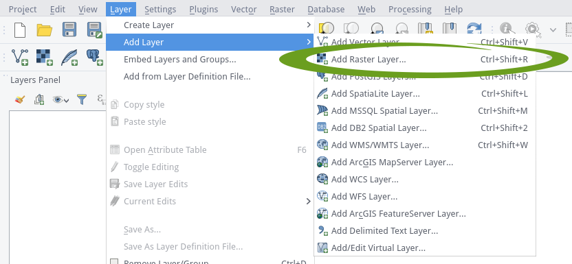
There are several ways to open a raster dataset here: Either navigate via the main menu to Layer > Add Layer > Add Raster Layer…, or press the corresponding icon in the toolbar or press the shortcut Ctrl + Shift + R to open a file explorer window.

In the file explorer window, navigate to the data folder which holds your L8 data and import a raster dataset. We will use a L8 scene showing Berlin (ID: LC08_L1TP_193023_20170602_20170615_01_T1) from the L8 Download Exercise. The spatial subset can be downloaded here directly:

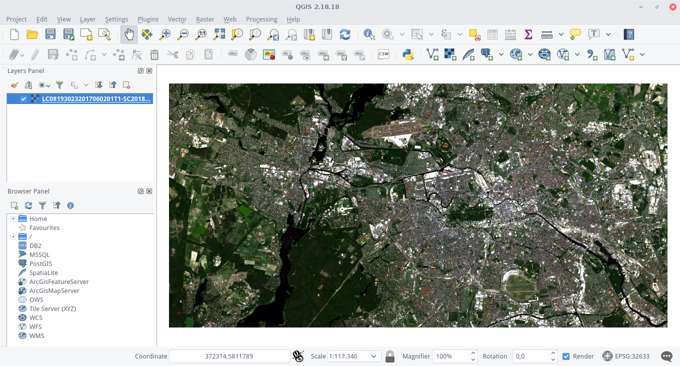
If you have started a new QGIS project (or just opened QGIS), the projection of the entire project will be based on the first dataset you load – in this case the raster file. You can see the current projection of the project in the lower right corner of QGIS. If you use our example data set, you should now see there. Click on this entry to get more detailed information about coordinate system of our raster dataset (“WGS84 / UTM ZONE 33 N”). Alternatively you can double-click the dataset in the Layer Panel and view the Coordinate Reference System (CRS) in the General-tab. We want to generate a new shapefile, which shares exactly this georeference system. This is the best way to ensure that the polygons are geographically correctly located in the end.

Create a New Polygon Shapefile

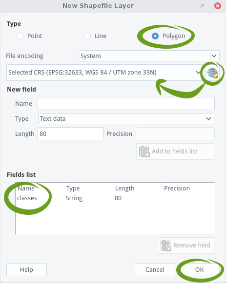
First, navigate to the area of interest (AOI) in your image data. Then click on the New Shapfile Layer icon in the toolbar. If you can not find this icon, right-click in the toolbar area and make sure there is a check mark next to “Manage Layer Toolbar”, which should reveal this icon among others. Once clicked, the “New Shapefile Layer” dialog will be displayed. Choose “polygon” as the Type in the top row of the window. Click on the Coordinate System icon. A new window will pup up, allowing you the choose the CRS of your new shapefile. Choose the same CRS as your raster data (you can use the filter function at the top). On the Fields list, select “id”, and click the button at the bottom of the list. Under “New field”, type “classes” in the Name box, click on . Finally, this should look like this:

If everything is set up, click OK. You will be prompted to the “Save layer as…” dialog. Type the file name (“training_data.shp”), choose a file path and click Save. You will be able to see the new shapefile in the Layers Panel of QGIS. Select it and press the Toggle Editing icon in order to activate editing functionalities. Note that a little pencil symbol will show up on top of the layer, indicating that the layer is now editable. Now click on the Add Feature icon. The mouse cursor will now look like a crosshairs. Left-click on the map in the Map View to create the first point of your new feature. Keep on left-clicking for each additional point you wish to include in your polygon. When you have finished adding your points, right-click anywhere on the map area to confirm your polygon geometry. An attribute window will appear immediately, asking for your class label. Input the appropriate class label for your polygon and click OK. Click on the Toggle Editing icon again in order to end editing and to save your changes by choosing Save.

You can edit the shape of a polygon with the Node tool . Delete any unwanted polygons by clicking on the tool called “Select Features by Area or Single Click” . Once activated you can left-click on polygons you want to delete, causing them to turn yellow. Then, press the delete key on your keyboard to remove the polygons (only in editing mode). Choose “Categorized” in the uppermost drop-down menu.

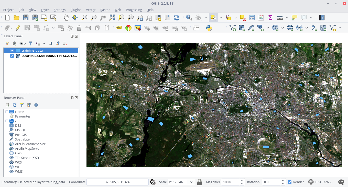
After some time you should have collected some training areas:

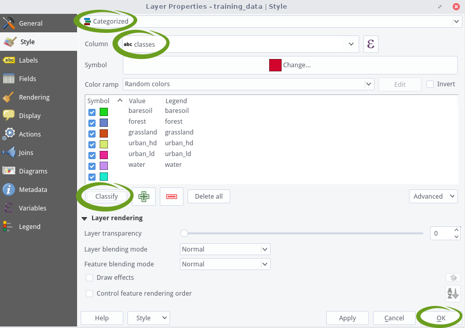
You can also color the polygons during editing based on the “classes” attribute, which makes it easier for you to estimate the class distribution. Double-click the shapefile in the Layers Panel and navigate to the Style tab. Ensure that your attribute “classes” is selected in the drop-down menu below. Click Classify once to apply an individual color to each class (click on the colored boxes in order to change the colors) and confirm everything by pressing OK:

If you think you have collected enough samples, save everything by clicking on the Toggle Editing icon again and choose to Save.
We do not need QGIS anymore, so close it.

---

NEXT
Prepare Samples in R