We want to create training samples in the form of a data frame – which most regressors in R can handle easily. For this we will have to use a few GIS operations. Fortunately, these can also be done automatically in R, so that the entire workflow do not have to be performed manually again and again for other datasets. Finally, we will utilize the raster and the rgeos packages for this.
The complete code is shown below. The shapefile reg_train_data.shp and the imagery LC081930232017060201T1-SC20180613160412_subset.tif can be downloaded here.
However, we strongly advise you to have a look at the detailed description in the following.
library(raster)
library(rgeos)

# import low resolution image and digitized polygon training areas
setwd("/media/sf_exchange/regression/")
img <- brick("LC081930232017060201T1-SC20180613160412_subset.tif")
shp <- shapefile("reg_train_data.shp")

# rename bands if needed
names(img) <- c("b1", "b2", "b3", "b4", "b5", "b6", "b7")
# create buffer with no width to avoid topology problems
shp <- gBuffer(shp, byid=TRUE, width=0)

# crop image to extent of training polygons
img.subset <- crop(img, shp)
# extract pixel completely covered by training polygons
img.mask <- rasterize(shp, img.subset, getCover = TRUE)
img.mask[img.mask < 100] <- NA
img.subset <- mask(img.subset, img.mask)
# transform those pixels to polygons
grid <- rasterToPolygons(img.subset)
# create a new ID attribute for addressing
grid$ID <- seq.int(nrow(grid))

# create new dataframe for final samples
smp <- data.frame()
# do for each cell in grid:
for (i in 1:length(grid)) {
  # intersect grid and shapefile for cell i
  cell <- intersect(grid[i, ], shp)
  # extract all target class polygons
  cell <- cell[cell$Class_name == "building" | cell$Class_name == "impervious", ]
  # if target class is in cell: calculate area, otherwise area is zero
  if (length(cell) > 0) {
    areaPercent <- sum(area(cell) / area(grid)[1])
  } else {
    areaPercent <- 0
  }
  # create new sample and append to training samples
  newsmp <- cbind(grid@data[i, 1:nlayers(img)], areaPercent)
  smp <- rbind(smp, newsmp)
}
In-depth Guide
In order to use functionalities of the raster and rgeos packages, load them into your current session via library(). If you do not use our VM, you must first download and install the packages with install.packages():
#install.packages("raster")
#install.packages("rgeos")
library(raster)
library(rgeos)
Next: set your working directory, in which all your image and shapefile data is stored by giving a character (do not forget the quotation marks ” “) variable to setwd(). Check your path with getwd() and the stored files in it via dir():
setwd("/media/sf_exchange/regression/")

getwd()
## [1] "/media/sf_exchange/regression"

dir()
##  [1] "LC081930232017060201T1-SC20180613160412_subset.tif"
##  [2] "reg_train_data.dbf"
##  [3] "reg_train_data.prj"
##  [4] "reg_train_data.qpj"
##  [5] "reg_train_data.shp"
##  [6] "reg_train_data.shx"
If you do not get your files listed, there is an error in your working path – check again! Everything ready to go? Fine, then import your raster file as img and your shapefile as shp and have a look at them:
img <- brick("LC081930232017060201T1-SC20180613160412_subset.tif")
img
## class       : RasterBrick
## dimensions  : 504, 1030, 519120, 7  (nrow, ncol, ncell, nlayers)
## resolution  : 30, 30  (x, y)
## extent      : 369795, 400695, 5812395, 5827515  (xmin, xmax, ymin, ymax)
## coord. ref. : +proj=utm +zone=33 +datum=WGS84 +units=m +no_defs +ellps=WGS84 +towgs84=0,0,0
## data source : /media/sf_exchange/regression/LC081930232017060201T1-SC20180613160412_subset.tif
## names       : LC0819302//2_subset.1, LC0819302//2_subset.2, LC0819302//2_subset.3, LC0819302//2_subset.4, LC0819302//2_subset.5, LC0819302//2_subset.6, LC0819302//2_subset.7
## min values  :                 -2000,                 -2000,                 -1502,                 -1384,                  -107,                   -72,                   -27
## max values  :                 13240,                 13539,                 14574,                 14549,                 14243,                 14896,                 15388

shp <- shapefile("reg_train_data.shp")
shp
## class       : SpatialPolygonsDataFrame
## features    : 286
## extent      : 390233.4, 390698.4, 5817147, 5817720  (xmin, xmax, ymin, ymax)
## coord. ref. : +proj=utm +zone=33 +datum=WGS84 +units=m +no_defs +ellps=WGS84 +towgs84=0,0,0
## variables   : 1
## names       : Class_name
## min values  :  bare_soil
## max values  :      water

compareCRS(shp, img)
## [1] TRUE
Both the brick() and shapefile() functions are provided by the raster package. As shown above, they create objects of the class RasterBrick and SpatialPolygonsDataFrame respectively. The L8 raster provides 7 bands, and our example shapefile 286 features, i.e., polygons. You can check whether the projections of the two datasets are identical or not by executing compareCRS(shp, img). If this is not the case (output equals FALSE), the raster package will automatically re-project your data on the fly later on. However, we recommend to adjust the projections manually in advance to prevent any future inaccuracies.
Plot your data to make sure everything is imported properly (check Visualize in R for an intro to plotting):
plot(shp)
With the argument add = TRUE in line 2 several data layers can be displayed one above the other:
plot(img[[4]], col=gray.colors(100))
plot(shp, add=TRUE)
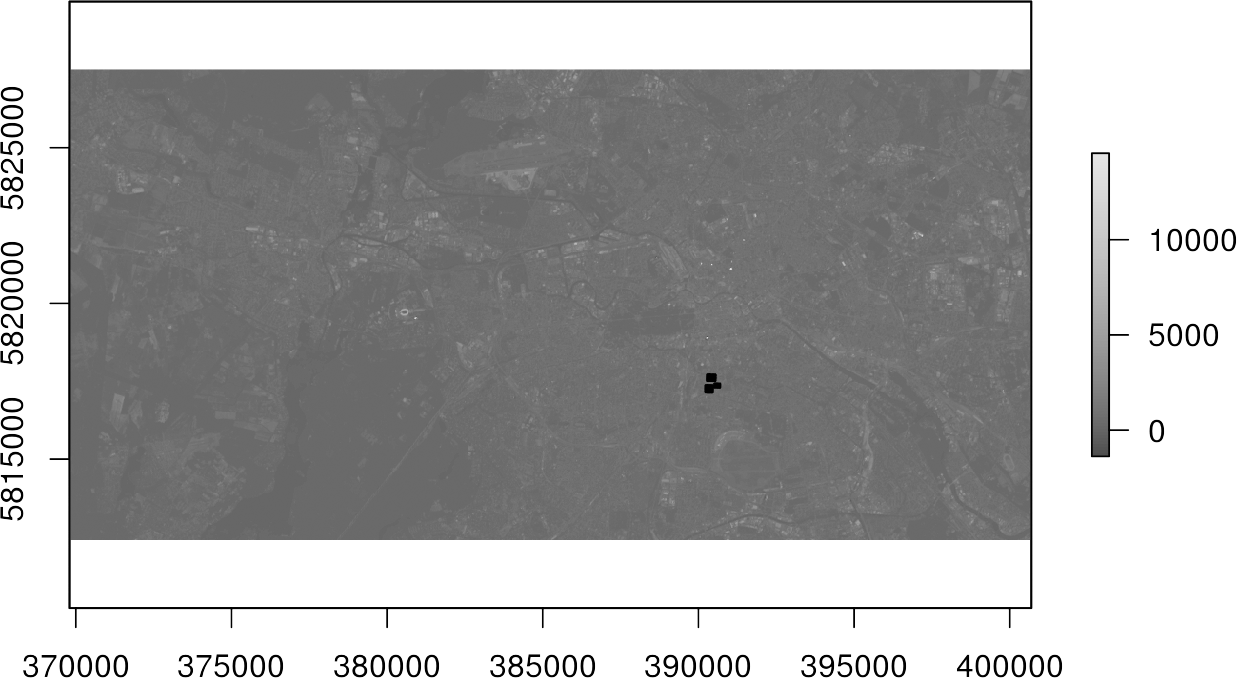
In Line 1, initially only the fourth channel of the image img[[4]] was displayed with a gray color representation using 100 shades col=gray.colors(100). The black spots in the upper plot represent the polygons of the shapefile. It becomes clear that they cover only a very small part of our study area.
Optional: Let us take a look at the naming of the raster bands via the names() function. Those names can be quite bulky and cause problems in some illustrations when used as axis labels. You can easily rename it to something more concise by overriding the names with any string vector of the same length:
names(img)
## [1] "LC081930232017060201T1.SC20180613160412_subset.1"
## [2] "LC081930232017060201T1.SC20180613160412_subset.2"
## [3] "LC081930232017060201T1.SC20180613160412_subset.3"
## [4] "LC081930232017060201T1.SC20180613160412_subset.4"
## [5] "LC081930232017060201T1.SC20180613160412_subset.5"
## [6] "LC081930232017060201T1.SC20180613160412_subset.6"
## [7] "LC081930232017060201T1.SC20180613160412_subset.7"

names(img) <- c("b1", "b2", "b3", "b4", "b5", "b6", "b7")

names(img)
## [1] "b1" "b2" "b3" "b4" "b5" "b6" "b7"
In order to accelerate all computation processes in the following, we first trim the image to the extent of the shapefile using the crop() function. It is often recommended to use a buffer of zero width wrapped around the polygons to avoid any topological errors in the upcoming process using gbuffer() as shown in line 1:
shp <- gBuffer(shp, byid=TRUE, width=0)

img.subset <- crop(img, shp)
Now we just want to extract the pixels that are 100% covered by the polygons. Full coverage is important to be able to extract reliable predictions about the ratio of an target class. In order to assess this coverage, we use the rasterize() function with the argument getCover = TRUE to generate a mask. In line 2, we set all pixels which have less than 100% coverage to NA. In the end, we use the mask to subset our image data again using the mask() function:
img.mask <- rasterize(shp, img.subset, getCover = TRUE)
img.mask[img.mask < 100] <- NA
img.subset <- mask(img.subset, img.mask)
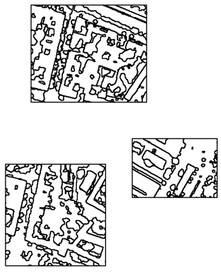
Plot the image data again with the polygons in order to see our achievements:
plot(shp)
plot(img.subset[[4]], add=T)
Only the raster cells within our polygons are left – great!
In a next step, we transform those pixels to polygons, forming a grid with the information of the Landsat 8 bands maintained by using the rasterToPolygons() function. In addition, we want to assign each of these cells in the grid with an ID in order to address them (line 2):
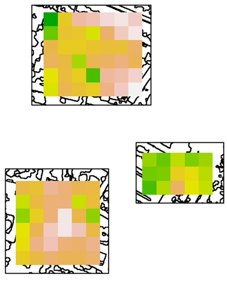
grid <- rasterToPolygons(img.subset)
grid$ID <- seq.int(nrow(grid))

grid
## class       : SpatialPolygonsDataFrame
## features    : 93
## extent      : 390255, 390675, 5817165, 5817705  (xmin, xmax, ymin, ymax)
## coord. ref. : +proj=utm +zone=33 +datum=WGS84 +units=m +no_defs +ellps=WGS84 +towgs84=0,0,0
## variables   : 8
## names       :   b1,   b2,   b3,   b4,   b5,   b6,   b7, ID
## min values  :  144,  198,  339,  279,  678,  563,  398,  1
## max values  : 1175, 1245, 1452, 1422, 3686, 2382, 2193, 93

plot(grid)

Finally, we have generated 93 cells (polygons) in this grid for which we now want to make a statement of how much of their areas is impervious, i.e., all polygons that have either building or impervious as Class_name attribute.
For this, we generate a new, empty data frame in which we write the training samples one after the other in line 1. We use a for-loop to iterate over each cell of the grid in line 2:
smp <- data.frame()
for (i in 1:length(grid)) {
  cell <- intersect(grid[i, ], shp)
  cell <- cell[cell$Class_name == "building" | cell$Class_name == "impervious", ]
  if (length(cell) > 0) {
    areaPercent <- sum(area(cell) / area(grid)[1])
  } else {
    areaPercent <- 0
  }
  newsmp <- cbind(grid@data[i, 1:nlayers(img)], areaPercent)
  smp <- rbind(smp, newsmp)
}

head(smp)
##      b1   b2   b3   b4   b5   b6  b7  areaPercent
## 2  1175 1245 1452 1422 1742 1321 950 9.765630e-01
## 3   497  597  736  767 1335 1175 947 7.986431e-01
## 5   277  330  477  462 1221  960 743 3.669043e-01
## 4   265  310  444  428 1077  789 545 1.727224e-01
## 41  230  267  390  343  809  613 404 9.765625e-06
## 42  168  217  339  312  678  563 398 3.540961e-02
Explanation:
Line 3: we select the ith cell of the grid and intersect this cell with the shp, which gives us the geometries and attributes of both the shapefile and the cell.
Line 4: only the polygons belonging to the target classes were extracted, we discard all other polygons.
Line 5: if a polygon of a target class exists in the cell, do everything inside the curly brackets. If there is no polygon in the cell, jump to line 7.
Line 6: calculate the proportion of the area of each polygon and sum the proportions (area(grid)[1] equals 900 m² in our example due to the geometric resolution).
Line 7: if there is no polygon of class building or impervious, set areaPercent to zero.
Line 10: use the column bind (cbind()) function to combine the feature values (reflectances of Landsat image) and the areaPercent value to form a new sample newsmp.
Line 10: use row bind (rbind()) to add the new sample newsmp to our training dataset smp.
We now prepared a training data set smp with all input features (Landsat 8 bands 1 to 7) and the percentage value of our target class (imperviousness).
Time to train a Support Vector Machine in the next section!