Alright, you have some image data now. The next step is to get an overview of the radiometric and geometric properties of the imagery you own. The comparison of several data sets is especially comfortable in QGIS with its overlay functionalities. However, we also want to take a closer look at the visualization capacities of R in order to achieve an optimal image presentation.

We will do some visualization settings on a Landsat 8 Scene data downloaded in the chapter Acquire. So if you have not done the exercises yet, catch it up here.

Visualization Basics

In the following basic concepts and terms are discussed and a understanding for the following section will be developed.

Singleband vs Multiband

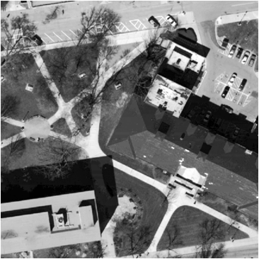
Most optical imaging satellite systems measure radiance in multiple spectral bands, including Landsat 8 and Sentinel 2 (see section Sensor Basics). As shown in the section Preprocess, these spectral bands are delivered as individual jpg- or tif-files within the data products. You can visualize each of those images separately by choosing a gray scale gradient (or any color slice). The following picture shows only the green band of an orthophoto of Berlin. Bright areas indicate high intensity of solar radiation reflected by the targets in the pixel, dark areas indicate low intensity:

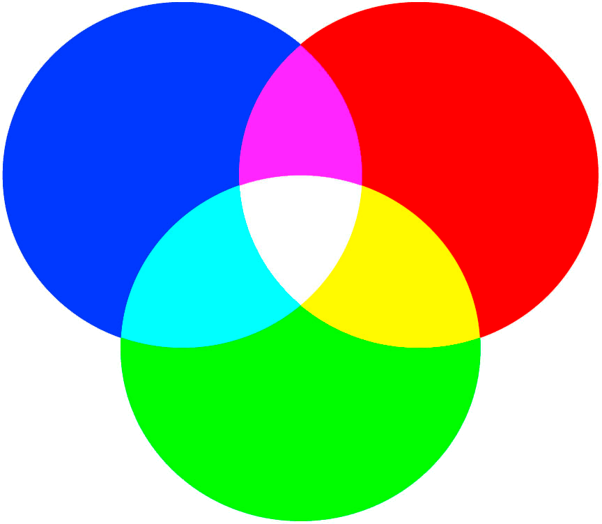
Such gray scale visualizations are useful for panchromatic bands, where only one band is available. However, this representation does not reflect what resembles the perception by the human eye. We are used to colorful pictures through our eyesight. On digital monitors, such as PC monitors, TV, or smartphones, this colorful display is achieved by mixing a number of different light colors, with shades of three primary colors: Red, Green and Blue. This method is called additive color mixing:

The same principle is used in the representation of satellite data: In the case of a colored RGB representation we have three “slots”: one for red, one for green and one for blue. If we fill each of these slots with a spectral channel of our satellite product, we will create a RGB composite due to the mixture of three different matrices of pixel values, i.e., digital numbers (DNs):

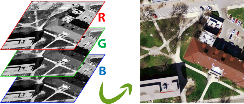
In this example, color representation is what we would assume: trees are green, footpaths are gray, and roofs are brown. This representation is called true-color composite and is achieved when the blue slot is occupied by the blue spectral band of the satellite sensor, the green slot with the green band and the red slot with the red band (have a look at the bands of L8 and S2 again!). Since sensors have far more spectral bands, there is a wide range of possible band combinations, so called false-color, or pseudocolor composites. Over time, some of these combinations have proven useful for specific issues:

BLUE	GREEN	RED	PURPOSE
blue	green	red	true color composite, the “nature color” combination
NIR	red	green	“false-colour” combination for vegetation, appears in shades of red
MIR	NIR	green	provides a “natural-like” rendition, penetrating atm. particles and smoke
NIR	MIR	red	offers added definition of land-water boundaries
NIR	MIR	blue	general great amount of information and color contrast

Histograms and Contrast Stretching

Each grayscale image consists of a 2-dimensional array, i.e, a matrix, of pixels that describe the intensities of the solar energy radiance measured by the sensor. These pixels are nothing more than integers and can be represented as such:

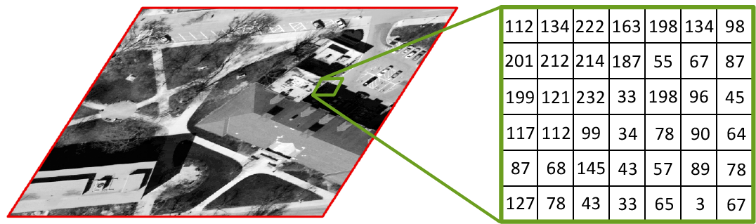
The occurrence of these integers can be counted and plotted. This representation is called a histogram and describes the frequency distribution of the gray level values in a single band image. A histogram shows the frequencies at the y-axis and the respective digital numbers (pixel values) at the x-axis:

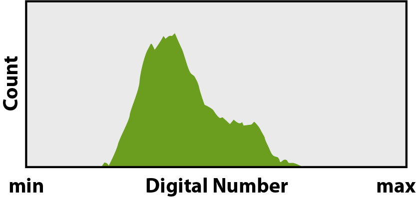
Histograms of optical images are typically normally distributed and thus unimodal. The range of digital numbers (min & max in the figure above) depends on the individual radiometric resolution of the data set, e.g., Landsat 8 Level-1 and Sentintel 2 Level-1 data provide 0 – 65,535 DNs (16 bit unsigned) and Landsat 8 Level-2 data provide −32,768 – 32,767 DNs (16 bit signed).
However, the complete range of theoretically possible digital numbers is rarely used by remote sensing imagery. As a consequence, images usually have a very low contrast when viewed in QGIS or R , whereby essential information remains hidden to us. The contrast of an image is a measure of its dynamic range, i.e., the spread of its histogram, and is calculated by the difference between maximum and minimum values of the image. A Minimum-Maximum contrast stretching increases the dynamic range by applying a linear scaling function that maps pixel values between the two extremes:

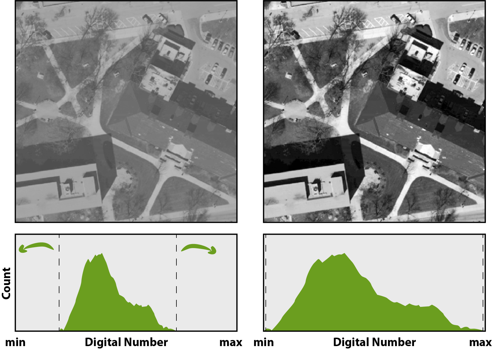
The image now takes on the full dynamic range and subjectively looks better to the human eye. The actual values of the dataset remain unaffected by any contrast stretching – it is only a modification for visual purposes. An underlying color or lookup table translates the original DNs to the stretched DNs. In addition to the Minimum-Maximum method, there are other stretch procedures available, such as Standard Deviations, Percent Clip or Sigmoid.

---

NEXT
Visualize in QGIS