The Random Forest (RF) algorithm is an all-rounder when it comes to data science problems!
Random Forests can be used for classification and regression tasks, while being non-linear and non-parametric, they can handle highdimensional, numerical and categorial variables and they have no special requirements or assumptions for the data to be used – so you do not have to worry about data distributing or standardizing your input features. And the best part: The basic concept is relatively easy to understand!

The RF is a representative of the so called “ensemble learning” methods. The word ensemble means nothing more than group in this context: A standard RF is based on generating a large number (ntree) of decision trees (DT) during the training phase (we will discuss those in a second), each constructed using a different subset (n) of your training dataset (N). Those subsets, also called bootstrap samples, are selected randomly and with replacement. After the training of the algorithm, each of those DTs is capable to map input data \(X\) (e.g., reflectances within Landsat 8 bands) to an ouput response \(y\) (e.g., class labels, like urban, water and forest). The Random Forest algorithm listens to all the responses of the DTs and make its final prediction on the basis of the most frequenty given response (majority vote). In case of regression, the RF takes the average of all the DT responses.
By growing multiple DTs, we can overcome or weaken the shortcomings of a single DT by combining them to form a more powerful model. Let us take a closer look at how a single decision tree works.

Decision Tree Method

A Decision Tree, also known as Classification and Regression Tree (CART), is a supervised learning algorithm first introduced by Breiman et al. in 1984. We want to focus on the implementation used by the R package randomForest, which we will use later in this section.

A CART trains by splitting all available samples into homogeneous sub-groups of high purity based on a most significant feature.
But one thing at a time…

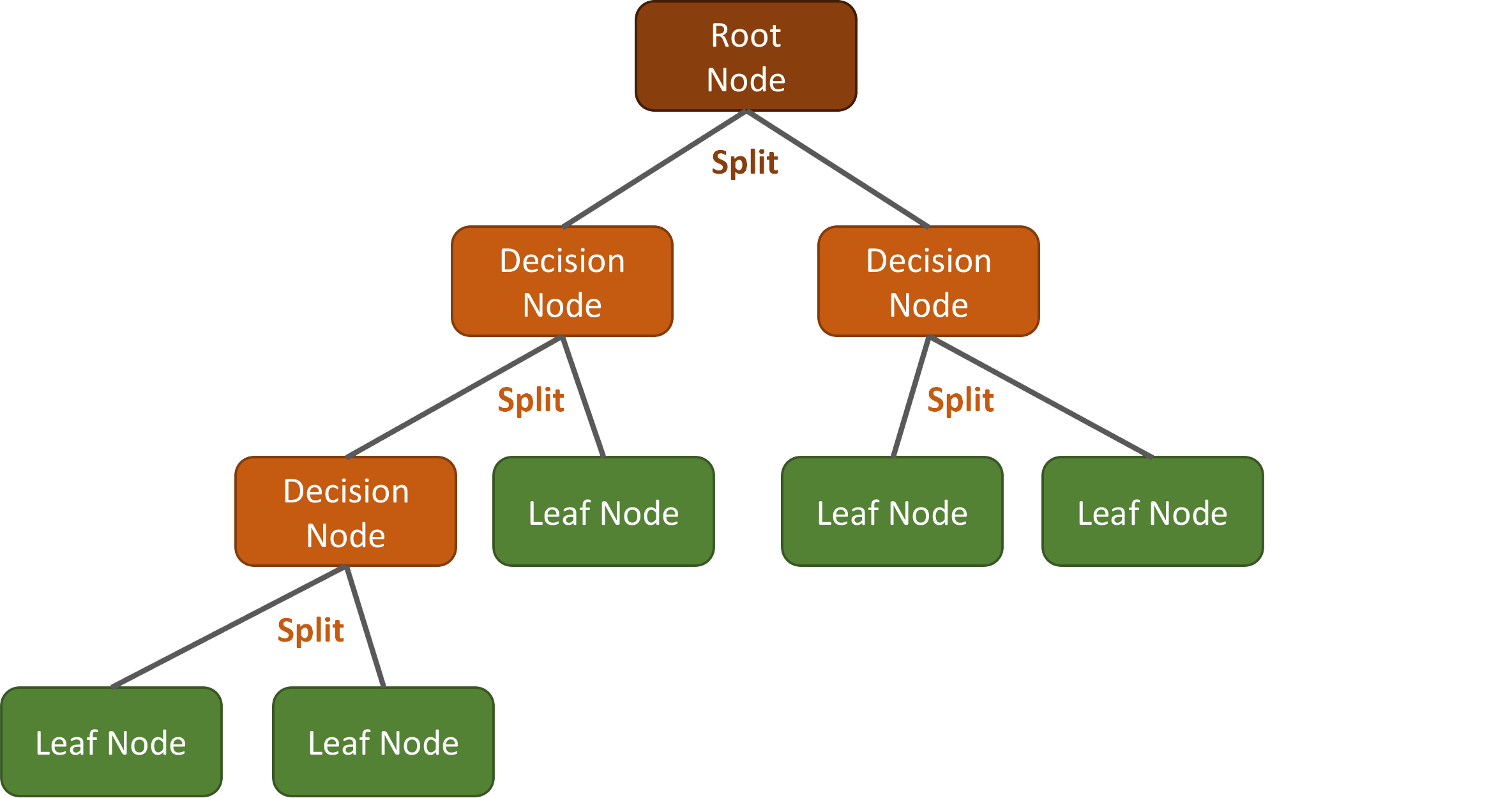
A decision tree conceptionally consists of three elements:

One Root Node: That is the starting point, which includes all training samples. A first split is done here.
Multiple Decision Nodes: Those are nodes where further splits are done.
Multiple Leaf (or Terminal) Nodes: Those are nodes where the assignments to the classes (e.g., urban, water, etc.) happens for classifications tasks (or the mean response of all observation in this node is calculated for regressions).

The structure and complexity of each DT can vary, depending on the training samples and the features used. For example, a very simple DT could look like this:

Ok, let us make that clearer with a fictitious example: We want to classify a Landsat 8 scene with 11 multispectral bands into four classes Forest, Urban, Bare Soil & Water. As a training dataset we use 500 pixels, 200 pixels belong to the forest class, 120 to urban, 80 to bare soil and to 100 water class, accordingly. We put all 500 samples in the Root Node in the top of the DT:

The next step is to split the node into two sub-nodes using a single threshold value. The CART algorithm always uses binary splits, i.e., it splits a node exactly in two sub-nodes, to increase the homogeneity of the resultant sub-nodes. In other words, it increases the purity of the node in respect to our target class. For example, the highest purity would be achieved if only one class was present in the first sub-node, and only one second class in the second sub-node. Of course this is not possible in our four class classification problem with only one split:

The first split could only clearly separate the Water samples, otherwise all classes are present at certain proportions in both subnodes. As you can see in the figure above, the DT decided to use the Landsat band 2 (b2) and the reflectance threshold value of 450 to do the split.

But wait a minute, how does the classifier know HOW and WHERE to do a split?!

The DT does not consider all features (Landsat bands) as candidates at each split, but only a certain number of features (\(mtry\)). By default, the parameter \(mtry\) corresponds to the root of the number of features \(M\) available, i.e., \(mtry = \sqrt{M}\). Thus, in our example the DT samples 3 out of 11 Landsat bands randomly and with replacement, because \(\sqrt{11}\approx3\).

There are various measures for determining the most significant candidate (e.g., Gini Index, Chi-Square, Variance Reduction or Information Gain). Our CART algorithm uses the Gini Index, so let us have a look at what it does:
Gini Index says, if we select two samples from our node, then they must be of the same class. If a node contains only one class, i.e., a completely pure node, Gini value would be 0. Thus, the lower the Gini value, the purer the node – which is good, because we want to group the samples according to their classes. The Gini Index is calculated by subtracting the sum of the squared probabilities \(p\) of each class \(\{1,2, …, C\}\) from one:

\begin{equation} \label{poly}\tag{1}
\text{Gini} = 1 – \sum_{i=1}^{C} (p^2).
\end{equation}

For the first split in our example shown in the figure above, the math would be:

calculate Gini for left sub-node: \((160/310)^2 + (40/310)^2 + (10/310)^2 + (100/310)^2 = 0.39\)
calculate Gini for right sub-node: \((40/190)^2 + (80/190)^2 + (70/190)^2 + (0/190)^2 = 0.36\)
calculate weighted Gini for split on feature (band 2): \((310/500) * 0.39 + (190/500) * 0.36 = 0.38\)

The Gini value is thus \(0.38\) if the Landsat Band 2 and the reflectance value 450 are chosen as as the feature and the threshold value, respectively. Finding a suitable threshold is an iterative process. So the algorithm tries many different values before picking out the one resulting in the smallest Gini, in this case the 450. As \(mtry = 3\) in our example, the DT will test two more bands, e.g., band11 and band 1, the same way and compare the Gini values in the end.

That is all the magic behind splitting procedure! In the same way, the sub-nodes are split further, making the tree “grow”:

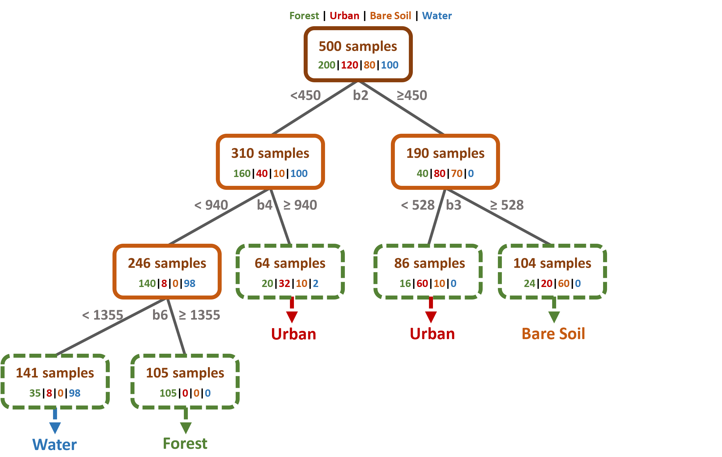
All samples within a leaf node are assigned to the class most frequently represented. The figure above shows, that the leaf nodes are not perfectly pure, e.g., there are 35 forest and 8 urban samples assigned to the water-node on the far left. These will result in misclassifications in your final classification map.

Working With Random Forests

In the case of a Random Forest approach, the tree shown above would continue growing until almost all nodes contain only one class at a time. While that would most likely result in overfitting in a single DT, this effect is relativized by the majority vote in the end when using a RF. Anyway, there are some more advantages when using a RF:

Out of Bag (OOB) Error:
There is no need for a cross-validation or a separate test set, as the OOB Error is estimated internally in the training phase as an unbiased estimate of the classification error. Remind: Each DT is created based on a small sample of your original training data (the so-called bootstrap sample). About one-third of the samples within this bootstrap sample are left out (out-of-bag) and not used for the construction of the DT. After the construction of the DT, the left out samples are used to test the tree. The Leaf Nodes then provide the class that is most represented by the OOB samples in each node. The proportion of samples that does not correspond to the class in the Leaf Node, averaged over all Leaf Nodes, is the OOB Error (overall accuracy for classifications and mean absolute error for regressions).

Variable Importance (VI)::
A RF can identify the most significant/ important features for your classification or regression task. Therefore it can also be considered as a method for dimensionality reduction.
If you plot the variable importance, you will get two measures in the randomforest package:
MeanDecreaseAccuracy: we permute all threshold values of a specific feature (e.g., Landsat band 2) and see how the purity in a Leaf Node changes. In detail: we count the number of correctly classified OOB samples once the tree is grown. After that, we randomly permutate the values of a specific feature for the OOB samples and classify the OOB samples again. The difference of correctly classified samples between permuted and original OOB data, averaged over all trees, is the MeanDecreaseAccuracy.
MeanDecreaseGini: each time a split is done, both sub-nodes become more pure and the Gini values decrease. The sum of all Gini decreases for each individual feature (e.g., Landsat band) over all trees is the MeanDecreaseAccuracy.