Just as with the Random Forest, there are quite a few R packages that provide SVM, e.g., caret, e1071, or kernLab. We will use the e1071 package, as it offers an interface to the well-known libsvm implementation.
Below you can see a complete code implementation. While this is already executable with your input data, you should read the comprehensive in-depth guide in the following to understand the code in detail.
# import packages
library(raster)
library(e1071)

# import image (img) and shapefile (shp)
setwd("/media/sf_exchange/landsatdata/")
img <- brick("LC081930232017060201T1-SC20180613160412_subset.tif")
shp <- shapefile("training_data.shp")

# extract samples with class labels and put them all together in a dataframe
names(img) <- c("b1", "b2", "b3", "b4", "b5", "b6", "b7")
smp <- extract(img, shp, df = TRUE)
smp$cl <- as.factor( shp$classes[ match(smp$ID, seq(nrow(shp)) ) ] )
smp <- smp[-1]

# optional: shuffle samples and undersample if necessary
smp <- smp[sample(nrow(smp)),]
smp <- smp[ave(1:(nrow(smp)), smp$cl, FUN = seq) <= min(summary(smp$cl)), ]

# tune and train model via gridsearch (gamma & cost)
gammas = 2^(-8:5)
costs = 2^(-5:8)
svmgs <- tune(svm,
              train.x = smp[-ncol(smp)],
              train.y = smp$cl,
              scale = TRUE,
              kernel = "radial",
              type = "C-classification",
              ranges = list(gamma = gammas,
                            cost = costs),
              tunecontrol = tune.control(cross = 5)
              )

# save svmmodel
svmmodel <- svmgs$best.model
save(svmmodel, file = "svmmodel.RData")

# predict image data with svm model
result <- predict(img,
                  svmmodel,
                  filename = "classification_svm.tif",
                  overwrite = TRUE
                  )
In-depth Guide
In order to be able to use the functions of the e1071 package, we must additionally load the library into the current session via library(). If you do not use our VM, you must first download and install the packages with install.packages():
#install.packages("raster")
#install.packages("e1071")
library(raster)
library(e1071)
First, it is necessary to process the training samples in the form of a data frame. The necessary steps are described in detail in the previous section.
names(img) <- c("b1", "b2", "b3", "b4", "b5", "b6", "b7")
smp <- extract(img, shp, df = TRUE)
smp$cl <- as.factor( shp$classes[ match(smp$ID, seq(nrow(shp)) ) ] )
smp <- smp[-1]
After that, you can identify the number of available training samples per class with summary(). There is often an imbalance in the number of those training pixels, i.e., one class is represented by a large number of pixels, while another class has very few samples:
summary(smp$cl)
##  baresoil    forest grassland  urban_hd  urban_ld     water
##       719      2074      1226      1284       969       763
This often leads to the problem that classifiers favor and overclass strongly-represented classes in the classification. Unfortunately, a SVM can not handle this problem as elegantly as Random Forest methods, why you might need to prepare your training data:
Only if your data is imbalanced, you should consider to do the following undersampling: We shuffle our entire training dataset and pick out the same number of samples for each class. The purpose of shuffle is to prevent sampling of all pixels that are next to each other (spatial autocorrelation). The training data is mixed using the sample() method. We sample all rows of our dataset nrow(smp) in a random manner in line 10:
head(smp)
##    b1  b2  b3  b4  b5  b6 b7    cl
## 1 192 229 321 204 161 100 72 water
## 2 179 203 233 130 156  93 68 water
## 3 189 221 272 164 173 109 81 water
## 4 159 179 188  97 125  63 40 water
## 5 171 194 203 116 146  82 56 water
## 6 164 188 196 108 138  71 51 water

smp <- smp[sample(nrow(smp)), ]

head(smp)
##       b1  b2  b3  b4   b5   b6   b7       cl
## 2024 176 195 324 234 2146 1022  479   forest
## 5545 409 517 844 988 3038 3005 1818 baresoil
## 2877 195 212 363 293 2500 1435  690   forest
## 6210 303 322 482 411 2465 1410  872 urban_hd
## 6613 367 418 672 600 2855 1876 1210 urban_ld
## 321  163 178 201 136  124   76   56    water
Compare the first six entries of the smp dataset before and after the command in line 10 using the head() function. You will notice that the order of the rows is shuffled!
With the min() function, we can select the minimum value from the class column’s summary and use the ave() function to make a selection of the same size for each class:
summary(smp$cl)
##  baresoil    forest grassland  urban_hd  urban_ld     water
##       719      2074      1226      1284       969       763

smp.maxsamplesize <- min(summary(smp$cl))
smp.maxsamplesize
## [1] 719

smp <- smp[ave(1:(nrow(smp)), smp$cl, FUN = seq) <= smp.maxsamplesize, ]

summary(smp$cl)
##  baresoil    forest grassland  urban_hd  urban_ld     water
##       719       719       719       719       719       719
Let the training begin!
Classifications using an SVM require two parameters: one gamma \(\gamma\) and one cost \(C\) value (for more details refer to the SVM section). These hyperparameters significantly determine the performance of the model. Finding the best hyparameters is not trivial and the best combination can not be determined in advance. Thus, we try to find the best combination by trial and error. Therefore, we create two vectors comprising all values that should be tried out:
gammas = 2^(-8:5)
gammas
##  [1]  0.00390625  0.00781250  0.01562500  0.03125000  0.06250000
##  [6]  0.12500000  0.25000000  0.50000000  1.00000000  2.00000000
## [11]  4.00000000  8.00000000 16.00000000 32.00000000

costs = 2^(-5:8)
costs
##  [1]   0.03125   0.06250   0.12500   0.25000   0.50000   1.00000   2.00000
##  [8]   4.00000   8.00000  16.00000  32.00000  64.00000 128.00000 256.00000
So we have 14 different values for \(\gamma\) and 14 different values for \(C\). Thus, the whole training process is done for 196 (14 * 14) models, often referred to as gridsearch. Conversely, this means that the more parameters we check, the longer the training process takes.
We start the training with the tune() function. We need to specify the training samples as train.x, i.e., all columns of our smp dataframe except the last one, and the corresponding class labels as train.y, i.e. the last column of our smp dataframe:
svmgs <- tune(svm,
              train.x = smp[-ncol(smp)],
              train.y = smp[ ncol(smp)],
              type = "C-classification",
              kernel = "radial",
              scale = TRUE,
              ranges = list(gamma = gammas, cost = costs),
              tunecontrol = tune.control(cross = 5)
              )
We have to set the type of the SVM to “C-classification” in line 4 in order to perform a classification task. Furthermore, we set the kernel used in training and predicting to a RBF kernel via “radial”. We set the argument scale to TRUE in order to initiate the z-transformation of our data. The argument ranges in line 7 takes a named list of parameter vectors spanning the sampling range. We put our gammas and costs vectors in this list. By using the tunecontrol argument in line 8, you can set k for the k-fold cross validation on the training data, which is necessary to assess the model performance.
Depending on the complexity of the data, this step may take some time. Once completed, you can check the output by calling the resultant object name:
svmgs
##
## Parameter tuning of 'svm':
##
## - sampling method: 5-fold cross validation
##
## - best parameters:
##  gamma cost
##      2    8
##
## - best performance: 0.02132796
In the course of the cross-validation, the overall accuracies were compared and the best parameters were determined: In our example, those are 2 and 8 for \(\gamma\) and \(C\), respectively. Furthermore, the error of the best model is displayed: 2.1% error rate (which is quite good!).
We can plot the errors of all 196 different hyperparameter combinations in the so called gridsearch using the standard plot() function:
plot(svmgs)
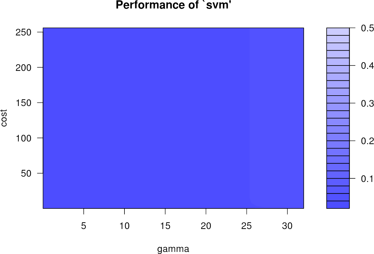
The plot appears very homogeneous, as the performance varies only very slightly and is already at a very high level. It can happen that the highest accuracies are found on the edge of the grid search. Then the training with other ranges for \(\gamma\) and \(C\) should be done again.
We can extract the best model out of our svmgs to use for image prediction:
svmmodel <- svmgs$best.model
svmmodel
##
## Call:
## best.tune(method = svm, train.x = smp[-ncol(smp)], train.y = smp$cl,
##     ranges = list(gamma = gammas, cost = costs), tunecontrol = tune.control(cross = 5),
##     scale = TRUE, kernel = "radial", type = "C-classification")
##
##
## Parameters:
##    SVM-Type:  C-classification
##  SVM-Kernel:  radial
##        cost:  8
##       gamma:  2
##
## Number of Support Vectors:  602
Save the best model by using the save() function. This function saves the model object svmmodel to your working directory, so that you have it permanently stored on your hard drive. If needed, you can load it any time with load().
save(svmmodel, file = "svmmodel.RData")
#load("svmmodel.RData")
Since your SVM model is now completely trained, you can use it to predict all the pixels in your image. The command method predict() takes a lot of work from you: It is recognized that there is an image which will be processed pixel by pixel. As with the training pixels, each image pixel is now individually classified and finally reassembled into your final classification image. Use the argument filename = to specify the name of your output map:
result <- predict(img,
svmmodel,
filename = "classification_svm.tif",
overwrite = TRUE
)
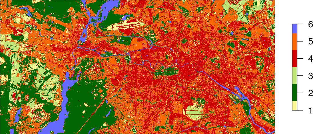
plot(result,
axes = FALSE,
box = FALSE,
col = c("#fbf793", # baresoil
"#006601", # forest
"#bfe578", # grassland
"#d00000", # urban_hd
"#fa6700", # urban_ld
"#6569ff" # water
)
)
Support Vector Machine classification completed!
If you store the result of the predict() function in an object, e.g., result, you can plot the map using the standard plot command and passing this object: