In this section we want to derive the Grey-Level Co-occurrence Matrix (GLCM) texture measurements for a S1 VH intensity raster. However, this workflow is not exclusive for Sentinel 1 data. You can derive GLCM metrics for any given raster, i.e., optical or radat. Due to the low spectral resolution and comparably low signal-to-noise ratio of radar data, the texture metrics are predestined to extend the feature space with meaningful data, e.g., for classification or regression tasks.
Luckily, the derivation of GLCM is done in one command in SNAP. Nevertheless, we want to create a graph file that theoretically allows you to process a lot of data easily via GPT. Have a look at the Bulk Processing Section of this course to learn, how to automate the process for many datasets.
Our workflow will contain the following sequential processing nodes:
- Read: Input – import a S1 scene (or any other raster file)
- GLCM: process all GLCM metrics of your choice
- Write: Output – write all GLCM bands into one GeoTiff raster file
Step by Step
First, get a pre-processed S1 image or another raster file of your study area. In the following example, we will use the VH-intensity image of a Sentinel 1 scene, which we derived in the previous section. You can download this example dataset here. It is not advantageous to use a speckle filter before deriving textures, as this eliminates most of the scene’s characteristics.
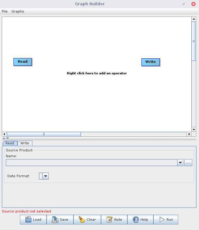
Open SNAP and click on the graph builder icon ![]() in the Toolbar. You will see a new window pop up, which shows a standard graph (containing one Read and one Write node) in the upper area and some options in the lower area.
in the Toolbar. You will see a new window pop up, which shows a standard graph (containing one Read and one Write node) in the upper area and some options in the lower area.
Right click somewhere in the white area in the upper window to add new nodes, i.e., processing steps, to the graph. Navigate to GLCM and add it:
- Read
- Add > Raster > Image Analysis > Texture Analysis > GLCM
- Write
Each processing step is visualized by a rectangle in the graph. You can drag those rectangles, or nodes, to whichever position you want with pressed left mouse button. Arrange the added nodes to something like this:
![]()
The individual nodes are not yet linked. If you rest the mouse pointer over the right edge of a rectangle, you will see a red arrow. Drag this arrow with pressed left mouse button to the next node in the following order:
![]()
Next, click on the Read Node and load your raster into the Source Product setting. This could take a short moment. Attention: From now on, it will always take a little while to switch back and forth between the processing nodes, as SNAP will process and read your data as virtual products in the background!
Now either click through the tabs at the bottom of the Graph Builder window or through the node rectangles to set the following options for all the nodes. You should try to make the settings in order, because graph building in SNAP is quite “fragile” and it may sometimes lead to strange errors, if the modules are not properly build on each other.
Parameters of GLCM:
Source Band: single input band of your raster, on which GLCM metrics should be derived
Window Size: moving window size for calulcating co-occurences
Angle: angle from which the neighborhood of two pixels is seen. Preferred: ALL
Quantizer: if probabilistic is selected, your GLCM matrix is expressed as probabilities instead of counting the total number of occurrences. Preferred: probabilistic
Quantization Levels: Number of gradations in the co-occurrence matrix (e.g., 32 different grey scale values). More quantized levels, less information loss. Less quantized levels, more information loss, but faster processing. Preferred: 32 or 64 levels
Displacement: Considered distance between two pixels. Distance of “1” means one pixel to the east from your reference pixel accounts for co-occurence statistics. Preferred: 1-4
When everything is set, you might want to save your graph. Simply click on “Save” on the bottom of the graph window and choose a file path. After that, start the graph via “Run”. Depending on the size of the study area and the processing nodes, this will take some time.
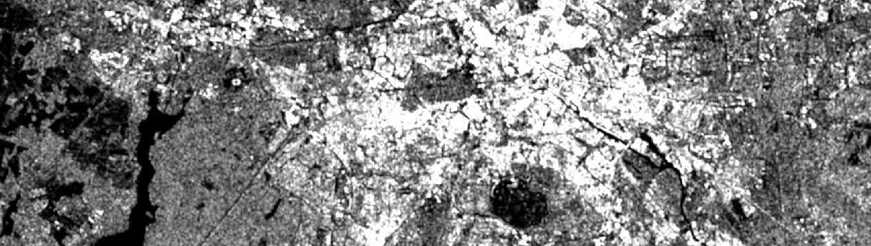
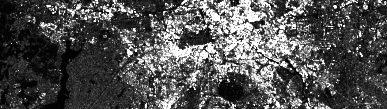
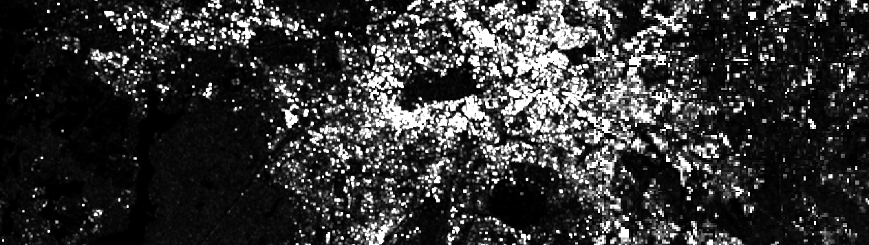
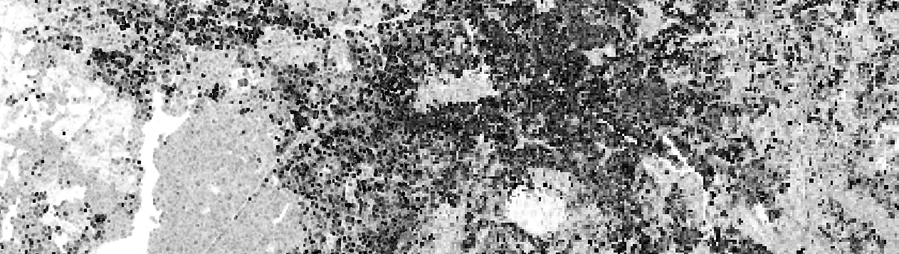
After processing is finished, you should get one GeoTiff-file that includes all selected metrics. Open the file in SNAP and double click the band you want to visualize:
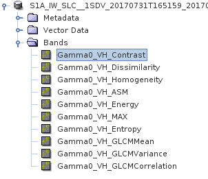
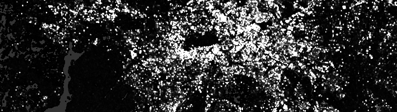
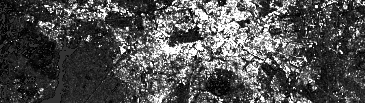
Those are the texture metrics opened in SNAP:
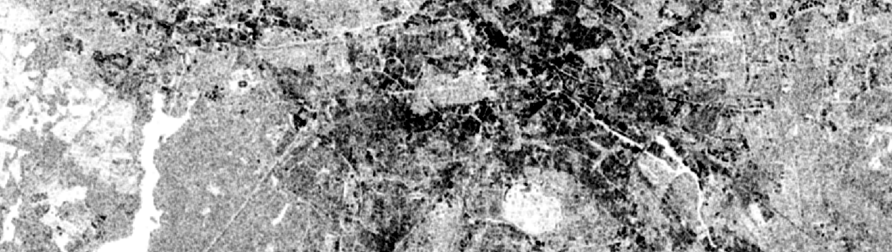
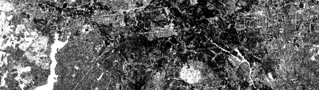
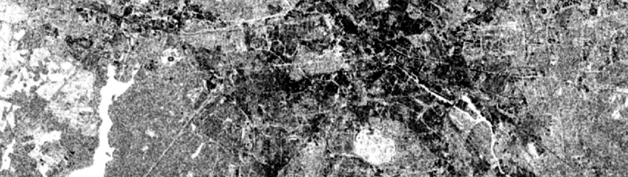
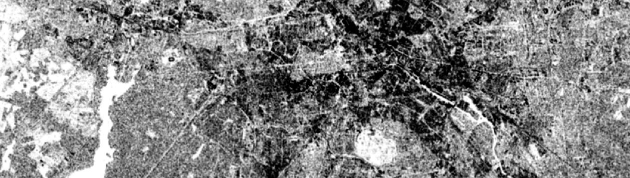
Haralick et al. 1973 or Hall-Beyer 2005