One question that is asked again and again is the amount of training data needed for a supervised classification. This question is not easy to answer, because every classification and regression problem is different.
However, there is an ideal analysis method to assess this problem for certain: creating a learning curve:
Simply repeat your training procedure multiple times with different train sample sizes and compare the performance differences!
Plotting those results will (hopefully) show a decreasing error rate with increasing amounts of train data.

In the following, a complete script has been developed, which performs the RF classification from the previous section with a maximum of \(\{2, 4, 8, 16, …, 2048\}\) samples per class (steps). In order to minimize any random effects and specify a confidence interval, all classifications were repeated 20 times each (nrepeat).

In order not to unnecessarily inflate the code, we use for loops to iterate over the individual sample sizes and iterations and write the respective results into a matrix r. The following code is comprehensively documented.

# import libraries
library(raster)
library(randomForest)

# import image (img) and shapefile (shp)
setwd("/media/sf_exchange/landsatdata/")
img <- brick("LC081930232017060201T1-SC20180613160412_subset.tif")
shp <- shapefile("training_data.shp")

# extract samples with class labels and put them all together in a dataframe
names(img) <- c("b1", "b2", "b3", "b4", "b5", "b6", "b7")
smp <- extract(img, shp, df = TRUE)
smp$cl <- as.factor(shp$classes[match(smp$ID, seq(nrow(shp)))])
smp <- smp[-1]

# number of samples per class chosen for each run
steps <- 2^(1:11)
# number of repetitions of each run
nrepeat = 20

# create empty matrix for final results
r <- matrix(0, 5, length(steps))

for (i in 1:length(steps)) {
  # create empty vector for OOB error from each repetition
  rtmp <- rep(0, nrepeat)
  
  for (j in 1:nrepeat) {
    # shuffle all samples and subset according to size defined in "steps"
    sub <- smp[sample(nrow(smp)),]
    sub <- sub[ave(1:(nrow(sub)), sub$cl, FUN = seq) <= steps[i], ]
    
    # RF classify as usual
    sub.size <- rep(min(summary(sub$cl)), nlevels(sub$cl))
    rfmodel <- tuneRF(x = sub[-ncol(sub)],
                      y = sub$cl,
                      sampsize = sub.size,
                      strata = sub$cl,
                      ntree = 250,
                      doBest = TRUE,plot = FALSE
                      )
    # extract OOB error rate of last tree (the longest trained) and save to rtmp
    ooberrors <- rfmodel$err.rate[ , 1]
    rtmp[j] <- ooberrors[length(ooberrors)]
  }
  
  # use repetitions to calc statistics (mean, min, max, CI) & save it to final results matrix
  ttest <- t.test(rtmp, conf.level = 0.95)
  r[ , i] <- c(mean(rtmp), ttest$conf.int[2], ttest$conf.int[1], max(rtmp), min(rtmp))
}

When the individual experiments have been processed, we can create a nice plot that summarizes the findings:

# conversion in percent
r <- r * 100
# plot empty plot without x-axis
plot(x = 1:length(steps),
     y = r[1,],
     ylim = c(min(r), max(r)),
     type = "n",
     xaxt = "n",
     xlab = "number of samples per class",
     ylab = "OOB error [%]"
     )
# complete the x-axis 
axis(1, at=1:length(steps), labels=steps)
# add a grid
grid()
# draw min-max range of OOB errors
polygon(c(1:length(steps), rev(1:length(steps))), 
        c(r[5, ], rev(r[4, ])),
        col = "grey80", 
        border = FALSE
        )
# draw confidence interval 95%
polygon(c(1:length(steps), rev(1:length(steps))), 
        c(r[3, ], rev(r[2, ])),
        col = "grey60", 
        border = FALSE
        )
# draw line of mean OOB 
lines(1:length(steps), r[1, ], lwd = 3)
# add a legend
legend("topright",
       c("mean", "t-test CI 95%", "min-max range"),
       col = c("black", "grey80", "grey60"),
       lwd = 3,
       bty = "n"
       )

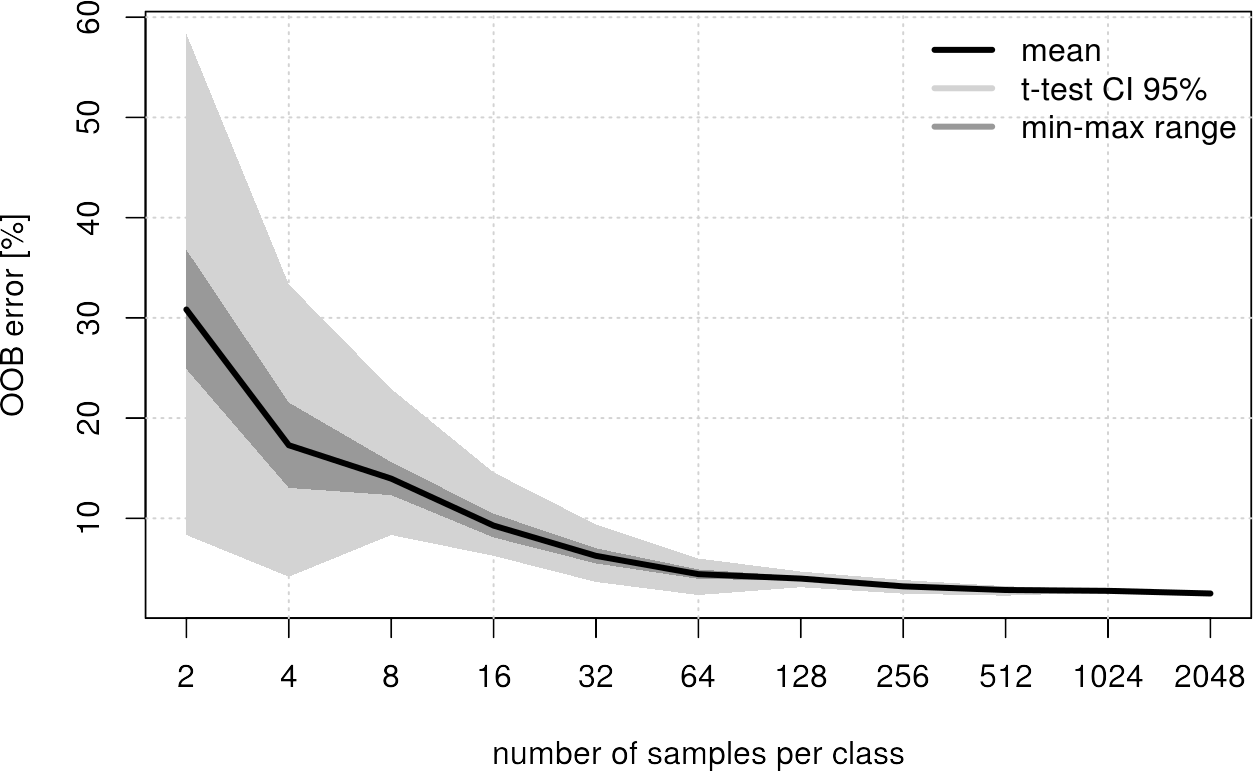
Conclusion for this example: From 512 samples per class the achieved improvement is negligible. So 512 samples per class should be enough to get a robust classification.

---

NEXT
Regression in R