There are several R packages that provide SVM regression, or Support Vector Regression (SVR), support, e.g., caret, e1071, or kernLab. We will use the e1071 package, as it offers an interface to the well-known libsvm implementation.
Below you can see a complete code implementation. Read the previous section to learn about pre-processing the training data. While this is already executable with the given input data, you should read the in-depth guide in the following to understand the code in detail.
# import
library(raster)
library(rgeos)
library(e1071)

setwd("/media/sf_exchange/regression/")
img <- brick("LC081930232017060201T1-SC20180613160412_subset.tif")
shp <- shapefile("reg_train_data.shp")

# training sample preprocessing (see last section for details)
names(img) <- c("b1", "b2", "b3", "b4", "b5", "b6", "b7")
shp <- gBuffer(shp, byid=TRUE, width=0)
img.subset <- crop(img, shp)
img.mask <- rasterize(shp, img.subset, getCover = TRUE)
img.mask[img.mask < 100] <- NA
img.subset <- mask(img.subset, img.mask)
grid <- rasterToPolygons(img.subset)
grid$ID <- seq.int(nrow(grid))

smp <- data.frame()
for (i in 1:length(grid)) {
  cell <- intersect(grid[i, ], shp)
  cell <- cell[cell$Class_name == "building" | cell$Class_name == "impervious", ]
  if (length(cell) > 0) {
    areaPercent <- sum(area(cell) / area(grid)[1])
  } else {
    areaPercent <- 0
  }
  newsmp <- cbind(grid@data[i, 1:nlayers(img)], areaPercent)
  smp <- rbind(smp, newsmp)
}

# model training
# define search ranges
gammas = 2^(-8:3)
costs = 2^(-5:8)
epsilons = c(0.1, 0.01, 0.001)
# start training via gridsearch
svmgs <- tune(svm,
              train.x = smp[-ncol(smp)],
              train.y = smp[ncol(smp)],
              type = "eps-regression",
              kernel = "radial",
              scale = TRUE,
              ranges = list(gamma = gammas, cost = costs, epsolon = epsilons),
              tunecontrol = tune.control(cross = 5)
              )

# pick best model
svrmodel <- svmgs$best.model

# use best model for prediciton
result[result < 0] = 1
result[result < 0] = 0
In-depth Guide
In order to be able to use the regression functions of the e1071 package, we must additionally load the library into the current session via library(). If you do not use our VM, you must first download and install the packages with install.packages():
#install.packages("raster")
#install.packages("rgeos")
#install.packages("e1071")
library(raster)
library(rgeos)
library(e1071)
First, it is necessary to process the training samples in the form of a data frame. The necessary steps are shown in line 10-31 and described in detail in the previous section.
After the preprocessing, we can train our Support Vector Regression with the training dataset smp. We will utilize an epsilon Support Vector Regressions, which requires three parameters: one gamma \(\gamma\) value, one cost \(C\) value as well as a epsilon \(\varepsilon\) value (for more details refer to the SVM section). These hyperparameters significantly determine the performance of the model. Finding the best hyparameters is not trivial and the best combination can not be determined in advance. Thus, we try to find the best combination iteratively by trial and error. Therefore, we create three vectors comprising all values that should be tested:
gammas = 2^(-8:3)
costs = 2^(-5:8)
epsilons = c(0.1, 0.01, 0.001)
So we have 14 different values for \(\gamma\), 14 different values for \(C\) and three different values for \(\varepsilon\). Thus, the whole training process is tested for 588 (14 * 14 * 3) models. Conversely, this means that the more parameters we check, the longer the training process takes.
We start the training with the tune() function. We need to specify the training samples as train.x, i.e., all columns of our smp dataframe except the last one, and the corresponding class labels as train.y, i.e. the last column of our smp dataframe, which holds the areaPercentageof our target class imperviousness:
svmgs <- tune(svm,
              train.x = smp[-ncol(smp)],
              train.y = smp[ncol(smp)],
              type = "eps-regression",
              kernel = "radial",
              scale = TRUE,
              ranges = list(gamma = gammas, cost = costs, epsolon = epsilons),
              tunecontrol = tune.control(cross = 5)
              )
We have to set the type of the SVM to “eps-regression” in line 4 in order to perform a regression task. Furthermore, we set the kernel used in training and predicting to a RBF kernel via “radial” (have a look at the SVM section for more details). We set the argument scale to TRUE in order to initiate the z-transformation of our data. The argument ranges in line 7 takes a named list of parameter vectors spanning the sampling range. We put our vectors gammas, costs and epsilons in this list. By using the tunecontrol argument in line 8, you can set k for the k-fold cross validation on the training data, which is necessary to assess the model performance.
Depending on the complexity of the data, this step may take some time. Once completed, you can check the output by calling the resultant object name:
svmgs
##
## Parameter tuning of ‘svm’:
##
## - sampling method: 5-fold cross validation
##
## - best parameters:
##       gamma cost epsolon
##  0.00390625    8     0.1
##
## - best performance: 0.03157376
In the course of the cross-validation, the overall accuracies were compared and the best parameters were determined: In our example, those are 0.0039, 8 and 0.1 for \(\gamma\), \(C\) and \(\varepsilon\), respectively. Furthermore, the Mean Absolute Error (MAE) of the best model is displayed, which is 0.0316, or 3.12%, in our case.
We can extract the best model out of our svmgs to use for image prediction:
svrmodel <- svmgs$best.model
svrmodel
##
## Call:
## best.tune(method = svm, train.x = smp[-ncol(smp)], train.y = smp[ncol(smp)], ranges = list(gamma = gammas, cost = costs,
##     epsolon = epsilons), tunecontrol = tune.control(cross = 5), type = "eps-regression", kernel = "radial", scale = TRUE)
##
##
## Parameters:
##    SVM-Type:  eps-regression
##  SVM-Kernel:  radial
##        cost:  8
##       gamma:  0.00390625
##     epsilon:  0.1
##
##
## Number of Support Vectors:  78
Save the best model by using the save() function. This function saves the model object svrmodel to your working directory, so that you have it permanently stored on your hard drive. If needed, you can load it any time with load().
save(svrmodel, file = "svrmodel.RData")
#load("svrmodel.RData")
Since your SVR model is now completely trained, you can use it to predict all the pixels in your image. The command method predict() takes a lot of work from you: It is recognized that there is an image which will be processed pixel by pixel. As with the training pixels, each image pixel is now individually regressed and finally reassembled into your final regression image. Save the output as raster object result and have a look at its minimum and maximum values (line 11):
result <- predict(img, svrmodel)

result
## class       : RasterLayer
## dimensions  : 504, 1030, 519120  (nrow, ncol, ncell)
## resolution  : 30, 30  (x, y)
## extent      : 369795, 400695, 5812395, 5827515  (xmin, xmax, ymin, ymax)
## coord. ref. : +proj=utm +zone=33 +datum=WGS84 +units=m +no_defs +ellps=WGS84 +towgs84=0,0,0
## data source : in memory
## names       : layer
## values      : -0.7562021, 1.15675  (min, max)
You may will notice some “super-positive” (values above 1.0 or 100%) and/ or some negative (values below 0.0 or 0%) values. Such values are not uncommon, since the SVR implementation of the e1071 package is not subject to any non-negative constraints. You could simply fix this issue by overriding all adequate entries with meaningful minimum and maximum values (0 for 0% and 1 for 100%) by adding the following two lines:
result[result > 1] = 1
result[result < 0] = 0
Finally, save your regression raster output using the writeRaster() function and plot your result in R:
writeRaster(result, filename="regression.tif")

plot(result, col=gray.colors(100))
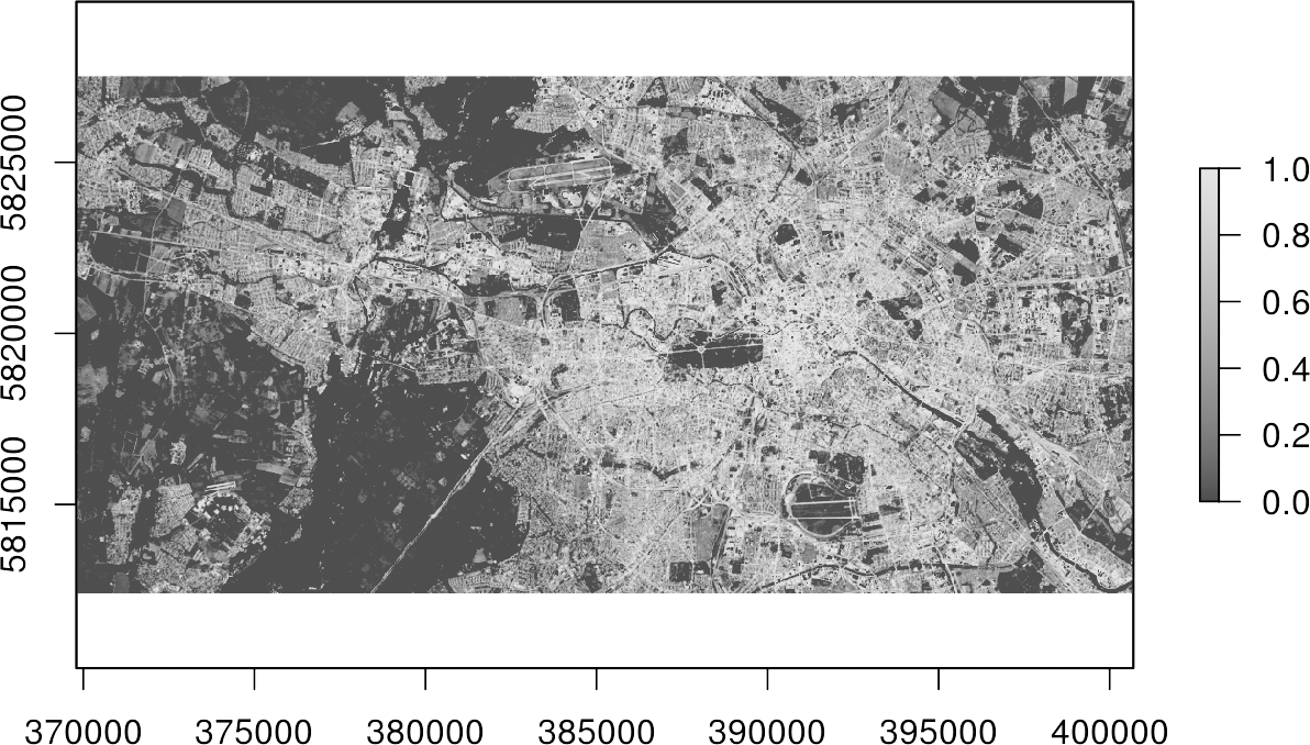
Done! You now got a map, which indicates the percentage of imperviousness, i.e., subpixel-information, for every single pixel in your image data.