This section contains advanced techniques. Understanding these techniques is particularly relevant if you want to pre-process dozens of Sentinel 2 data in an identical way.
We will create a graph in SNAP and then modify it to process all data automatically via the Graph Processing Tool (GPT)!

Open SNAP and click on the graph builder icon in the Toolbar. You will see a new window pop up, which shows a standard graph (containing one Read and one Write node) in the upper area and some options in the lower area. Right click somewhere in the white area at upper window to add new nodes, i.e., processing steps, to the graph. Navigate to Add > Raster > Geometric > Resample to add an Resample and a Subset node (those are the steps we used in the above section):

Each processing step is visualized by a rectangle in the graph. You can drag those rectangles, or nodes, to whichever position you want with pressed left mouse button. Your graph should now look something like this:

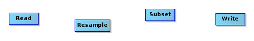
The individual nodes are not yet linked. If you rest the mouse pointer over the right edge of a rectangle, you will see a red arrow. Drag this arrow with pressed left mouse button to the next node in the following order:

Next, click on the Read Node and load one of your ZIP-compressed Sentinel 2 scenes into the Source Product setting. This could take a short moment. Attention: From now on, it will always take a little while to switch back and forth between the processing nodes, as SNAP will process and read your data as virtual products in the background!

Now either click through the tabs at the bottom of the Graph Builder window or through the rectangles at the top to set the following options for the Resampling, the Subset and the Write node (according to the settings made in the previous section):

The spatial section in the Subset node should be made using the geographic coordinates. However, the linked map is quite blurred and therefore not much help. However, under the map you can define any spatial subset using the Well-Known Text (WKT) format. There are a number of simple online tools for creating such WKTs. Copy the entire “Polygon(())” expression into the line below the map within the subset Node:

POLYGON((13.11 52.65, 13.70 52.65, 13.70 52.35, 13.11 52.35, 13.11 52.65))

Of course, you can add more processing steps later for your own analysis. When you are done click Save on the bottom of the Graph Builder window and save your graph as “myGraph.xml” to your hard drive (exchange folder recommended):

Automate Things Using GPT

Close SNAP, as we do not need it anymore. Now, open a terminal, which is linked in the taskbar of our VM:

It is possible to run the graph using the GPT now. The GPT can be found in our VM in the file path “/home/student/snap/bin/gpt”. Consequently, we can execute the graph with the following command (change the file path corresponding to the location of your graph file!):

/home/student/snap/bin/gpt /media/sf_exchange/sentineldata/myGraph.xml

Replace the path with the path of your file, copy it to the terminal and press Enter!

A pre-processed file should be created directly in the same folder as your zip-compressed source file.
However, you can only process one file with the graph so far… That is not exactly what we wanted. That is why we will make some changes to the xml-file now. Right click the xml-file and choose Open With > Open With “Text Editor”. Take a moment to understand how the file is structured. The individual inputs and outputs of all processes, or nodes, are saved here as a text. Each of the successive processes is opened by a <node = id “”> tag and closed by /node> .
Search for the Read node. Within that node, a line should list the Sentinel 2 file you used when creating the graph (the line number may differ in your xml):

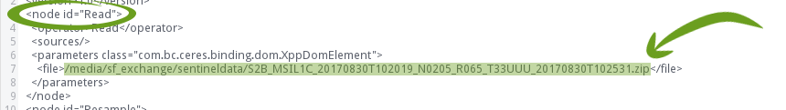
Replace the filename (marked green in the figure above) with the placeholder $input:

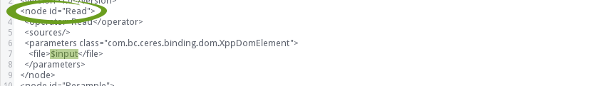
Now search for the Write node:

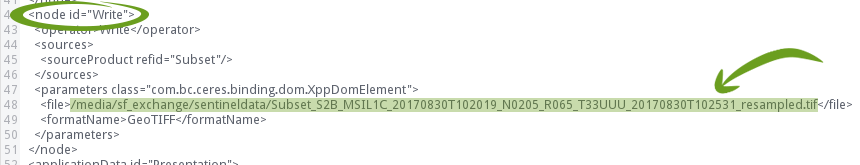
And replace the file path with the placeholder $output:

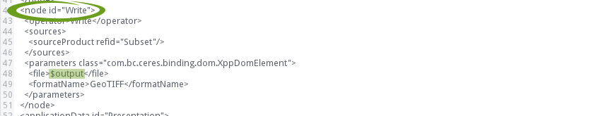
The input and output paths have now been replaced by placeholders, which could dynamically accept any file. When calling the graph via GPT, the two variables $input and $output must always be defined with from now on. A possible call for a file might look like this:

/home/student/snap/bin/gpt /media/sf_exchange/sentineldata/myGraph.xml -Pinput=/media/sf_exchange/sentineldata/S2B_MSIL1C_20170830T102019_N0205_R065_T33UUU_20170830T102531.zip -Poutput=/media/sf_exchange/sentineldata/S2B_MSIL1C_20170830T102019_N0205_R065_T33UUU_20170830T102531_sub_res.tif

Of course, we can take advantage of this and use a for-loop to go through and process all the Sentinel 2 datasets located in a folder one after another using R or a bash script. We have prepared a bash script for you, which does just that, located in /home/student/Documents/S2_proc.bash. This script tells the bash shell of Linux what it has to do, so you will need our VM or any Linux operating system. To run the script, open a terminal, reference the script and give it two arguments: first the full path to your graph .xml file and second the path where the downloaded Sentinel 2 zip-files are located. A possible command might look like this:

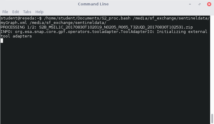
/home/student/Documents/S2_proc.bash /media/sf_exchange/sentineldata/myGraph.xml /media/sf_exchange/sentineldata/

The script starts as soon as you press enter and writes the output to a new folder called “Processed”, which will be created next to your S2 zip files.

 

---